

The summer of 2026 has been exceptionally warm and dry across much of Europe, with several record-breaking heatwaves. The first episode began in late May, when many national and local May maximum-temperature records were broken across western Europe. A second heatwave developed over western Europe in late June, before shifting eastward, breaking all-time temperature records in several central and northern European countries. July remained warm and very dry across much of western and central Europe, contributing to drought conditions, very low flows in major rivers such as the Rhine and Danube, and numerous wildfires. At the time of writing, another record-breaking heatwave is affecting central Europe. A summary of climate indicators for July 2026 can be found in the Copernicus Climate Change climate bulletin.
Sub-seasonal predictions
Figure 1 compares May to July mean temperature anomalies in ERA5 with composites of sub-seasonal forecasts at lead times of 2, 3 and 6 weeks, based on weekly anomalies for 4 May to 2 August. ERA5 shows warm anomalies across much of western Europe, strongest over northern France, where the three-month anomaly reached about 3°C. Conditions were closer to normal over northern and eastern Europe. The week-2 and week-3 forecasts captured the broad western European warm signal, although the week-3 forecast incorrectly predicted anomalous warmth over Scandinavia. By week-6, the warm signal covered most of Europe but was displaced eastward. The corresponding precipitation diagnostic (not shown here) indicates a strong dry anomaly across much of Europe, except in Scandinavia and north-eastern Europe. This pattern was reasonably well predicted at weeks 2 and 3, and even the week-6 mean retained a weak signal of the contrast between dry central Europe and wet western Scandinavia.
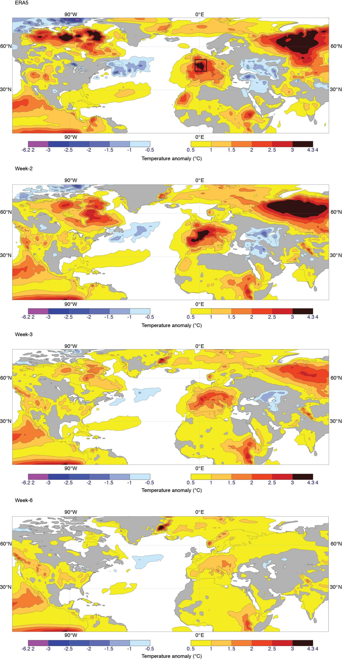
Figure 1 Average temperature anomalies in ERA5 (top panel) and composites of sub-seasonal forecasts at lead times of 2, 3 and 6 weeks (lower three panels), based on weekly anomalies for 4 May–2 August. The box in the top panel indicates the area over France used for the analysis shown in Figure 2.
Figure 2 shows weekly temperature anomalies from ERA5 and ensemble-mean sub-seasonal forecasts at different lead times for a box covering most of France (see box in Figure 1, top panel). ERA5 and the week-1 forecasts captured the late-May and late-June heatwaves, the persistent positive anomalies during July, and the cold start to May. The week-2 forecasts captured the timing of the main warm peaks but missed both the early-May cold anomaly and the break between the May and June heatwaves. At longer lead times, the forecasts became progressively warmer as the season developed but provided little guidance on intra-seasonal variability. This increasing warm signal may be a consequence of increasingly dry initial conditions.
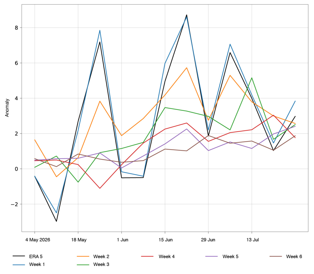
Figure 2 Weekly temperature anomalies from ERA5 and ensemble-mean sub-seasonal forecasts at different lead times, averaged over a box covering most of France (see Figure 1, top panel).
Heatwave forecast examples
Figure 3 shows the forecast evolution for 2-metre temperature in two heatwave cases: a 0.5° × 0.5° box centred on London Heathrow at 12 UTC on 26 May, and a corresponding box around Angers, France, at 12 UTC on 24 June. The use of 12 UTC temperature, rather than daily maximum temperature, is due to the current lack of daily maximum output from the Artificial Intelligence Forecasting System (AIFS). In both cases, short-range AIFS forecasts, including deterministic and ensemble configurations, were warmer than the corresponding Integrated Forecasting System (IFS) forecasts and closer to observations. In the medium range, both ensembles had a warmer-than-normal signal as early as 15 days before the event that gradually increased in strength. Around 5 to 8 days ahead, the AIFS ensemble gave a stronger signal than the IFS ensemble for both cases. Whether this reflects better prediction of the synoptic state or better representation of near-surface temperature extremes requires further investigation.
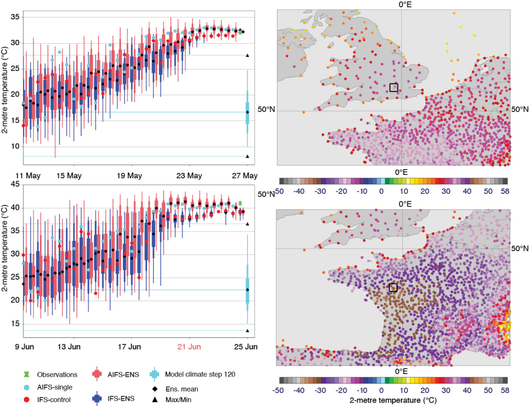
Figure 3 Forecast evolution for 2-metre temperature for 0.5° × 0.5° boxes centred on London Heathrow at 12 UTC on 26 May (top) and around Angers, France, at 12 UTC on 24 June 2026 (bottom). Corresponding observations are shown on the right.
Two-metre temperature bias
To place the short-range 12 UTC temperature differences between the IFS and AIFS in context, Figure 4 shows day-2 two-metre temperature bias over Europe for May to July for the IFS control forecast and the AIFS, for forecasts verifying at 00 UTC and 12 UTC. The discussion focuses on regions north and west of the Alps, while noting that large biases occur elsewhere. Because the verification period was anomalously warm, longer lead times would be expected to be cold on average through loss of predictability. A two-day lead time is therefore used to retain well-predicted synoptic conditions while exposing local systematic errors. At 12 UTC, the IFS has a stronger cold bias than the AIFS over France. Farther east, for example over Germany, the picture is different and the AIFS instead shows a stronger warm bias. At 00 UTC, both models show a warm bias, with substantial local variation.
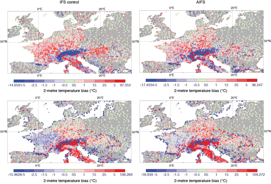
Figure 4 Day-2 two-metre temperature bias over Europe for May–July for the IFS control forecast (left) and the AIFS (right), for forecasts verifying at 00 UTC (top) and 12 UTC (bottom).
Summary
In summary, the sub-seasonal forecasts at week-3 and beyond captured a warmer-than-normal signal for weeks that verified in July but missed the early-summer heatwaves. Medium-range predictability was initially limited, although signals began to emerge in both IFS and AIFS ensemble forecasts about two weeks before the event peaked.
In the short range, the IFS underestimated the absolute magnitude of the highest temperatures, whereas the AIFS appears to have captured them more accurately. Underestimation of maximum temperature during heatwaves is a long-standing IFS deficiency that has been investigated several times, although no clear cause has yet been identified.
Although the AIFS outperformed the IFS in these examples, both in medium-range signal strength and near-surface temperature magnitude, several components are still needed before it can support key operational products. AIFS re-forecasts are required for Extreme Forecast Index (EFI) plots and for the model climatology used in 15-day meteograms. In addition, current AIFS output is available only every 6 hours, which is insufficient for estimating daily maximum and minimum temperatures. A time interpolator to provide hourly output is under development and is planned be included in a coming AIFS version. Work is also under way on a hybrid ensemble that nudges large-scale AIFS patterns into the IFS ensemble, providing the same output as the current IFS ensemble. Finally, a sub-seasonal AIFS forecasting system is under development.