In 1997, the incremental four-dimensional variational (4D-Var) data assimilation system became operational at ECMWF. 4D-Var is the system used at ECMWF to combine a short-range forecast with observations to produce the best possible estimate of the current state of the atmosphere. This then provides the initial conditions for a new forecast. The system works by minimising a cost function, which measures the departure of the analysis from observations and the short-range forecast. In this minimisation, linearised versions of the forecast model are used to efficiently determine the optimal 3D representation of the atmospheric state at a given time. From the very beginning, it was recognised that it is crucial to represent physical processes in the linearised model. Parametrization schemes used in linearised models have gradually become more and more complex. Nowadays, comprehensive schemes are included in ECMWF’s 4D-Var system. Recent data assimilation tests using the latest version of the linearised physics have again demonstrated a systematic and significant improvement for all parameters, levels, and regions.
Principles
At ECMWF, the 4D‑Var analysis system is employed to generate 3D atmospheric states (or analyses) which, together with separately produced land and ocean conditions, can be then used to initialise the Earth system model. This system uses the model dynamics and physics in an optimisation procedure, which aims to improve the overall fit of initial conditions to the observations available inside the assimilation time window, while staying as close as possible to the model first guess (a short-range forecast which forms the starting point in creating the analysis) in poorly observed regions. For more details see Box A.
A
4D-Var methodology
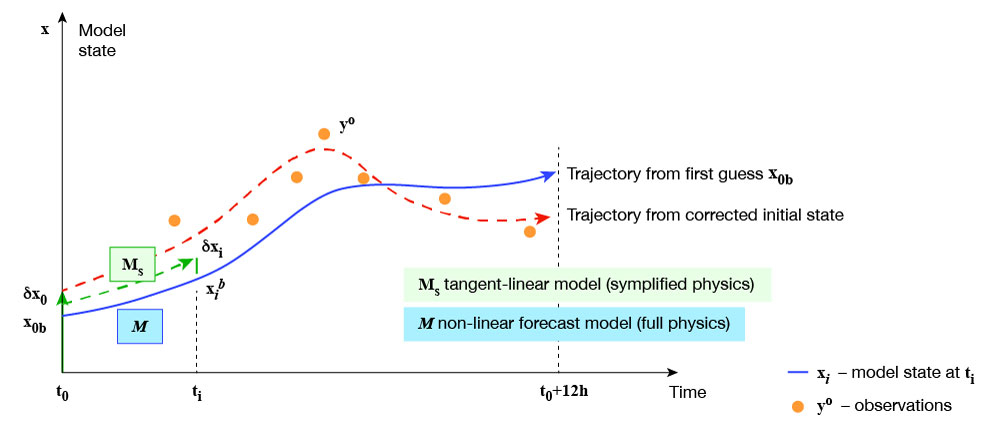
The goal of 4D‑Var is to define the initial atmospheric state such that its distance to the original model trajectory on the one hand and to the observations on the other is as small as possible over the assimilation time window (see the figure in this box).
At ECMWF, an incremental approach is used as a cost-effective formulation of 4D‑Var (Courtier et al., 1994). Using the incremental formulation, the model state at any time is defined in terms of an increment, i.e. a small perturbation around the background state (typically, a previous short-range forecast). To the first order, the 4D-Var problem can be solved by finding the analysis increment δx0 at initial time t0 which minimises the following cost function:

At any time ti , δxi = xi - xib is the analysis increment representing the departure of the model state (x) with respect to the background (xb), which consists of temperature, humidity, vorticity, divergence and surface pressure in the current 4D-Var system. di = yio – Hi (xib) is the so-called innovation vector, which provides the departure of the model background equivalent (Hi (xib)) from the observation (yio). Hi is the linearised observation operator (also describing the spatial interpolations to the observation locations and the forecast model integration propagating the initial state x0 to the time of observation). Ri is the observation-error covariance matrix (including measurement and representativeness errors) and B is the background-error covariance matrix of the state xb.
The minimisation requires an estimate of the gradient of the cost function:

where MT is the adjoint of the forecast model M and HT is the adjoint of the observation operator H, as explained in Box B.
The incremental approach reduces the computational cost of 4D‑Var since the perturbations δxi and the gradient of the cost function are computed at a lower resolution using the simplified model during successive minimisations (currently four at ECMWF). After each minimisation, the model trajectory is recomputed at high resolution.
In operational practice, innovation vectors are computed with the nonlinear model at high resolution including full physics. Increments are computed with the tangent-linear model at low resolution including simplified physics. The gradient of the cost function is computed with the low-resolution adjoint model using simplified physics.
4D‑Var relies on linearised versions of the forecast model, namely its tangent linear and adjoint versions (see Box B), to describe the time evolution of small perturbations around the reference state, typically in terms of temperature, wind, humidity and surface pressure.
B
Tangent-linear (TL) and adjoint (AD) models
If the model M describes the time evolution of the model state x from time ti to time ti+1 as:

the time evolution of a small perturbation δx can be estimated to the first order approximation by the tangent-linear version M of the non-linear model M:

The adjoint of the linear operator M is the linear operator M* such that:

where 〈 , 〉 denotes the inner product and x, y are randomly chosen input vectors. The adjoint operator, for the simplest canonical scalar product 〈 , 〉 in Eq. (5), is actually the transpose of the tangent linear operator, MT.
Variational assimilation is based on the adjoint technique, since the adjoint model MT can provide the gradient of any objective (cost) function, J, with respect to x(ti ) from the gradient of the objective (cost) function with respect to x(ti+1):

The integration of the AD forecast model works backward in time and all adjoint equations in the code are in reverse order compared to the tangent-linear equations.
In the 1980s, when experimentation and developments towards 4D‑Var data assimilation were under way, only the adiabatic version (i.e. dynamics only) of the linearised models was used. However, the importance of representing physical processes was soon recognised. It started to become obvious that the mismatch between the model analysis and observations can remain large during the 4D‑Var minimisation when only the adiabatic linearised model is used to evolve the model state from the beginning of the assimilation window to the time of each observation. Besides, without the inclusion of physics in variational data assimilation, the assimilation of many satellite observations, such as all‑sky radiances, precipitation and cloud-affected measurements, would simply be impossible.
ECMWF linearised physics
Although already started in the mid-1990s, the development of the linearised physics (LP) really gathered pace at the turn of the century, with the operational implementation of 4D‑Var.
At ECMWF, parametrization schemes for linearised models started from very simple ones. They aimed to remove very large increments, especially those produced close to the surface by the adiabatic model (Buizza, 1994). More complex but still incomplete schemes were then developed by Mahfouf (1999). Over the following years, more comprehensive schemes were gradually implemented. This led to a set of schemes able to describe most physical processes and their interactions with almost as much detail as in the non-linear model, but with just slight simplifications and/or regularisations (Janisková et al., 2002; Tompkins & Janisková, 2004; Lopez & Moreau, 2005).
The current set of physical parametrizations used in ECMWF’s linearised model (called simplified or linearised parametrizations hereafter) comprises six different schemes: radiation, vertical diffusion, orographic gravity wave drag, moist convection, large-scale condensation/precipitation and non-orographic gravity wave activity. The schemes are sequentially called in this order (Janisková & Lopez, 2013). This LP package is quite sophisticated and is believed to be the most comprehensive one currently in use for operational global data assimilation.
Developing and testing the linearised model
The construction of the linearised model starts with the design of a set of suitable non-linear physical parametrizations, from which the tangent-linear and adjoint versions can be derived. Thus, the whole development is rather demanding since it requires a good knowledge of both physical parametrizations and the adjoint. The validation must be very thorough, and it must be performed for the non-linear, tangent-linear and adjoint versions of the physical parametrization schemes.
Building the linearised model: a tricky compromise
In the real world, physical processes can be highly non-linear (NL) and often discontinuous. Since 4D-Var relies on the linearity assumption, it is necessary to either discard processes which could lead to instabilities, or to apply some regularisation to smooth the parametrizations’ discontinuities and render the schemes as differentiable as possible. Another constraint when developing parametrization schemes for data assimilation is related to the minimisation of the 4D‑Var cost function, which is solved with an iterative and therefore computationally demanding algorithm. Because of the constraints related to linearity and computational cost, the full NL model needs to be simplified before its successful inclusion in 4D‑Var computations. However, at the same time, parametrization schemes used in the linearised model must maintain a realistic representation of physical processes and remain as close as possible to the reference full NL model.
Once the simplified code is developed, it is necessary to tune and validate it. This is done by evaluating short forecasts (typically 12 hours; the length of the 4D‑Var time window) to ensure that the new simplified scheme is stable and does not depart too much from its full NL counterpart over the targeted integration period.
Tangent-linear approximation and regularisation
The tangent-linear (TL) model is used in 4D‑Var to evolve increments of the model state in time, from the beginning of the assimilation window to the time of the observations.
To build the tangent-linear model, a linearisation is performed with respect to the local tangent of the model trajectory. For the validation of the TL approximation, the accuracy of the linearisation is evaluated using pairs of two non‑linear 12‑hour forecasts. First the difference between two non-linear integrations (one starting from a background field and the other one starting from the corresponding analysis) is computed with the full NL model taken as a reference. Then a corresponding TL integration calculates the time evolution of the analysis increments (the difference between the analysis and the background field), with the trajectory being taken from the background field. The TL integration can then be compared with the NL difference to assess how well the TL model approximates its full NL counterpart. For a quantitative evaluation of the impact of linearised schemes, mean absolute errors between TL and NL integrations are computed. The mean absolute error for the TL model without physics (i.e. the adiabatic TL model) is usually taken as a reference in these comparisons.
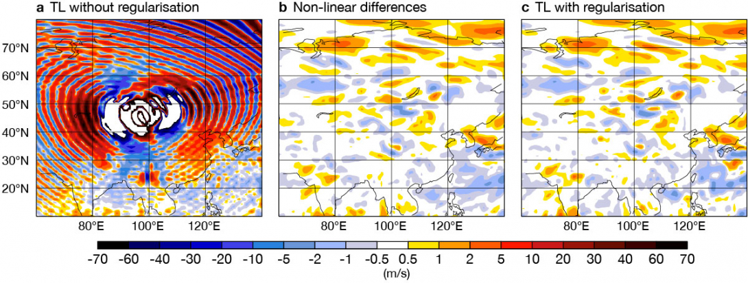
In some situations in which strong nonlinearities are present, especially when physical processes are included, special care must be taken to avoid the spurious development of perturbations in the linearised model. Without a proper treatment of the most significant nonlinearities and thresholds, the TL model can quickly become too inaccurate to be useful. Figure 1 illustrates some erroneous behaviour of the TL model due to too large local derivatives in the linearised model. When using the TL model without any regularisation in the orographic gravity wave drag scheme, strong spurious noise develops in the TL model (Figure 1a) compared to the differences between two NL integrations (Figure 1b). When regularisation is applied (consisting here in retaining the low-level blocking, while significantly reducing contributions from all other sub-grid scale orographic effects), TL increments (Figure 1c) agree well with the NL differences.
The impact of the LP on the TL approximation is illustrated in Figure 2. It shows the zonal mean cross-section of the change in TL error for temperature when the full LP is included in the TL model relative to the adiabatic TL model. The TL error is significantly reduced almost everywhere when physics is included in the linearised model. The largest improvement is observed in the lower troposphere, where many physical processes are active. Similarly, when looking at mean vertical profiles of the change in the TL error (Figure 3), there is a clear improvement for all variables (temperature, zonal and meridional wind, and humidity) and throughout the vertical.
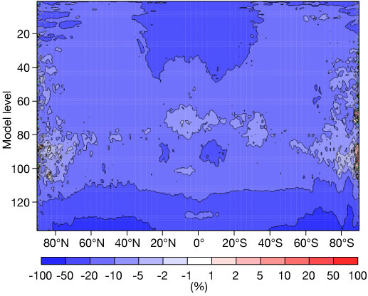
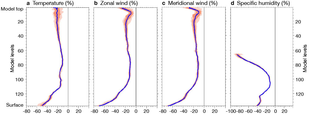
As illustrated, the TL model describing the evolution of perturbations, with simplified physical parametrizations included, generally fits the corresponding NL differences much better than the adiabatic TL model, provided discontinuities in the different physical parametrizations are properly smoothed. However, a regular effort is needed to ensure that the linearised model remains stable and noise-free in all meteorological situations, and after any modifications to the full NL model or to the TL model itself, or any change in the computing environment.
Adjoint test
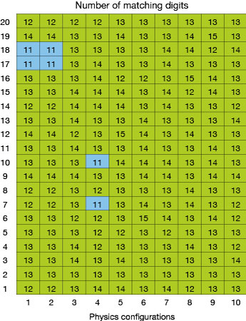
In variational data assimilation, the adjoint version of the TL model (which includes physical parametrizations at ECMWF) is used to estimate the gradient of the cost function to be minimised. The correctness of the adjoint must always be thoroughly checked by testing the identity described in Equation 5 (Box B). In this test, the TL and AD codes must agree to the level of machine precision, as illustrated in Figure 4. This test must be satisfied for global 3D atmospheric states and for integrations up to 12 hours (i.e. the maximum length of the 4D‑Var window at ECMWF). Achieving a correct adjoint test can be really time-consuming, as even the tiniest error in the code will make the test fail. It should be emphasised that the correctness of the adjoint test does not guarantee the correctness of the tangent-linear code. It only indicates that the adjoint is correct with respect to the TL code from which it was derived.
Impact of the linearised physics on 4D-Var analysis and forecast
The incremental impact of any change of the model’s physics on both TL approximation and on the performance of ECMWF’s Integrated Forecasting System (IFS) is regularly evaluated for every new model cycle. However, it has been a decade since the last time the impact on forecast skill from including the full linearised physics package in the 4D‑Var minimisation was assessed (Janisková & Lopez, 2013). Since then, several updates have been made to the linearised model to follow the changes of the full NL model. For instance, the cloud and convective schemes were significantly modified, and a simplified linearised parametrization of surface processes was implemented. Other adjustments were also required to deal with additional problems due to non-linearities and discontinuities in the parametrization schemes, which resulted from the increase in the horizontal and vertical resolutions of the model.
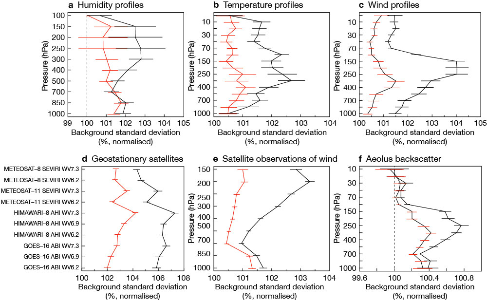
To evaluate the impact of the latest whole linearised physics package, three experiments have been performed for the period of July–September 2021, using IFS Cycle 47r3 at resolution TCo639 L137, corresponding to a horizontal resolution of approximately 18 km and 137 model levels in the vertical. 4D‑Var had inner loops at resolution T159, T191 and T255, corresponding approximately to 130 km, 100 km and 80 km respectively, and L137. The first experiment included the linearised physics and all observations as used in operations (reference); the second one excluded all observations (mostly precipitation and cloud-affected) which could not be used without the linearised physics in 4D‑Var; the third one also excluded the whole linearised physics.
The impact of including physical processes in the linearised model on 4D‑Var analyses was assessed by comparing the first guess fit to assimilated observations. The results are shown in Figure 5 both for conventional observations (humidity and temperature profiles as well as wind observations) and for selected satellite observations (satellite observations of wind and Aeolus satellite backscatter). They clearly indicate that the inclusion of LP in data assimilation provides significantly better 4D-Var analyses.
Furthermore, the impact on forecast scores coming from including the linearised physics in the 4D‑Var system is illustrated in Figure 6. The systematic and significant improvement for all parameters, levels and regions is clear. As expected, the impact of the LP in 4D‑Var is largest close to analysis time. The positive impact is highly remarkable, especially in the tropics. Overall, these results demonstrate the vital role of the LP in the 4D‑Var system, not only through its own huge positive impact, but also because it allows the assimilation of a whole range of observations which strongly rely on information provided by physical parametrizations, such as cloud, precipitations and surface parameters.

Conclusion
Including physical parametrization schemes in the linearised model clearly brings a large positive and significant impact in the data assimilation system at ECMWF. The inclusion of LP in 4D‑Var is essential not only to improve the realism of 4D‑Var increments, but also to assimilate observations that are highly sensitive to physical processes (e.g. cloud, precipitation, surface temperature and moisture). Therefore, proper maintenance and development of the LP will be an absolute prerequisite to the longevity of 4D‑Var, unless a competitive alternative can be found. For instance, ECMWF is looking at the potential role of machine learning emulators in the EU-funded MAELSTROM project.
Developing well-behaved and efficient linearised physics can be a complex and demanding task. For any new or major revision to a parametrization, a substantial amount of work can be required to simplify and regularise the code so that discontinuities and nonlinearities are eliminated or smoothed out. It is also essential to verify that the TL approximation is not degraded whenever a physical parametrization is modified, or the model horizontal or vertical resolution is changed, and to swiftly address any deterioration through appropriate updates to the TL and AD codes.
To maintain the best analysis and forecast performance possible, the best compromise between the constraints of linearity and computational cost on the one hand and realism on the other must be achieved. Increasingly complex parametrizations in the nonlinear model and increasing model and data assimilation resolution make maintaining the LP package challenging. However, these results demonstrate the considerable benefit to forecast skill achieved by continuing to meet these challenges.
Further reading
Buizza, R., 1994: Impact of simple vertical diffusion and of the optimisation time on optimal unstable structures. ECMWF Technical Memorandum, No. 192.
Courtier, P., J.-N. Thépaut & A. Hollingsworth, 1994: A strategy for operational implementation of 4DVar using an incremental approach. Q. J. R. Meteorol. Soc., 120, 1367–1387.
Janisková, M., J.-F. Mahfouf, J.-J. Morcrette & F. Chevallier, 2002: Linearised radiation and cloud schemes in the ECMWF model: Development and evaluation. Q. J. R. Meteorol. Soc., 128, 1505–1527.
Janisková, M. & P. Lopez, 2013: Linearised physics for data assimilation at ECMWF. In: S.K. Park and L. Xu (eds.), Data assimilation for Atmospheric, Oceanic and Hydrological Applications (Vol. II), https://doi.org/10.1007/978-3-642-35088-7, Springer-Verlag Berlin Heidelberg, 251–286.
Lopez, P. & E. Moreau, 2005: A convection scheme for data assimilation: description and initial tests. Q. J. R. Meteorol. Soc., 131, 409–436.
Mahfouf, J.-F., 1999: Influence of physical processes on the tangent-linear approximation. Tellus, 51, 147–166.
Tompkins, A.M. & M. Janisková, 2004: A cloud scheme for data assimilation: description and initial tests. Q. J. R. Meteorol. Soc., 130, 2495–2517.