Arctic weather forecasting – in the high Arctic

In spring 2018, scientists from several nations and a number of different projects were getting instruments and systems ready for the Arctic Ocean 2018 (AO2018) expedition on the Swedish research icebreaker Oden. Oden was heading for the high Arctic during August and September. The main goal was to investigate the formation and life cycle of low-level Arctic clouds (Box A). One of the projects participating in this expedition was Arctic Climate Across Scales (ACAS), funded by the Swedish Knut and Alice Wallenberg Foundation and endorsed by the Year of Polar Prediction (YOPP). One of the aims of this project is to increase the amount of meteorological observations from the sparsely observed central Arctic Ocean (Box B). The idea is to help advance numerical weather prediction and climate modelling by developing a quasi-unattended meteorological observatory on Oden. The need for minimal human intervention stems from the fact that the primary limitation for participating in icebreaker-based research is the limited number of berths on board the icebreakers that are used as platforms. As a contribution to YOPP, and in collaboration with the EU-funded Horizon 2020 project APPLICATE, we have begun to evaluate ECMWF operational forecasts in the Arctic using these observations from ACAS. Initial findings suggest that wind forecasts are of high quality but that there are some issues with cloudiness and temperature forecasts.

Expedition trajectory

Oden left Longyearbyen on Svalbard on 1 August, reached the North Pole on 12 August and, a few days later, moored to an ice floe about 2 km² in size near 89.5°N and 30°E. The ship drifted with this ice floe for a month, facilitating observations on the ice in addition to those taken on board. The expedition ended back in Longyearbyen on 21 September (Figure 1). The researchers used the almost stationary ice drift period, from 15 August to 14 September, to collect data for the forecast evaluation.

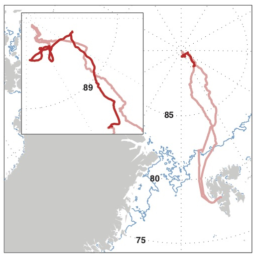
Ice conditions in early August along the northward track (Figure 1) were unexpectedly difficult. Although the ice edge was located unusually far north of Svalbard, the ice was thick and there was very little open water between ice floes once inside the pack ice. Such open water is a key factor for icebreaking. There were also a larger-than-expected number of icebergs all the way to the pole. A persistent high-pressure ridge during early August likely contributed to strong ice convergence, which created the harsh icebreaking conditions. The increased mobility of the ice probably resulted in the large number of icebergs, which must have come from land. During the ice camp, expedition members named a nearby iceberg Mt John, after the meteorological research engineer who was the first to climb it and who raised the Union Jack at its top.

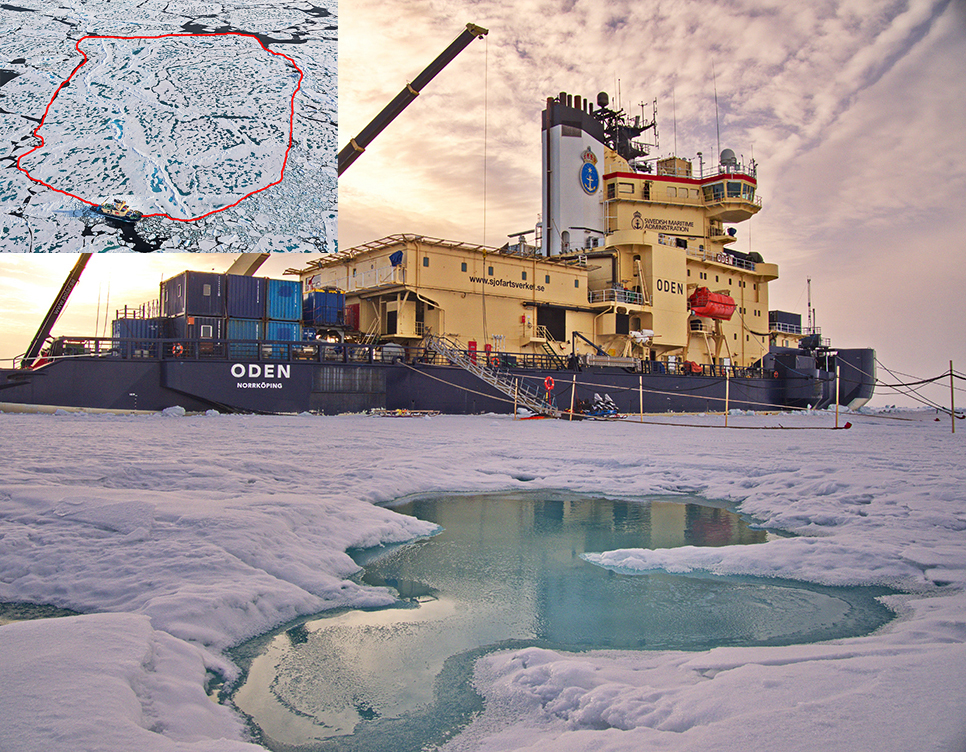
The weather was typical for the Arctic Ocean summer, with a lot of low cloud and fog. Throughout the expedition, fog prevailed for about 25% of the time, the average cloud fraction was close to 90%, and the lowest cloud base typically around 100 m. There was melting snow on the ice almost all the time until the end of August, when the summer melt ended, ensuring a high surface albedo in spite of many melt ponds (see Figure 2). Hence, on the few occasions when the clouds broke up and the sun came out, the change in surface net shortwave radiation was unable to balance the longwave cooling, causing the temperature to drop. This special condition applies through most of the summer over sea ice in the high Arctic. Near-surface temperature rarely goes above zero while the surface is melting. When the sun comes out, people can feel its warmth due to darker-coloured clothes, but the temperature typically plummets.

On-board forecasting

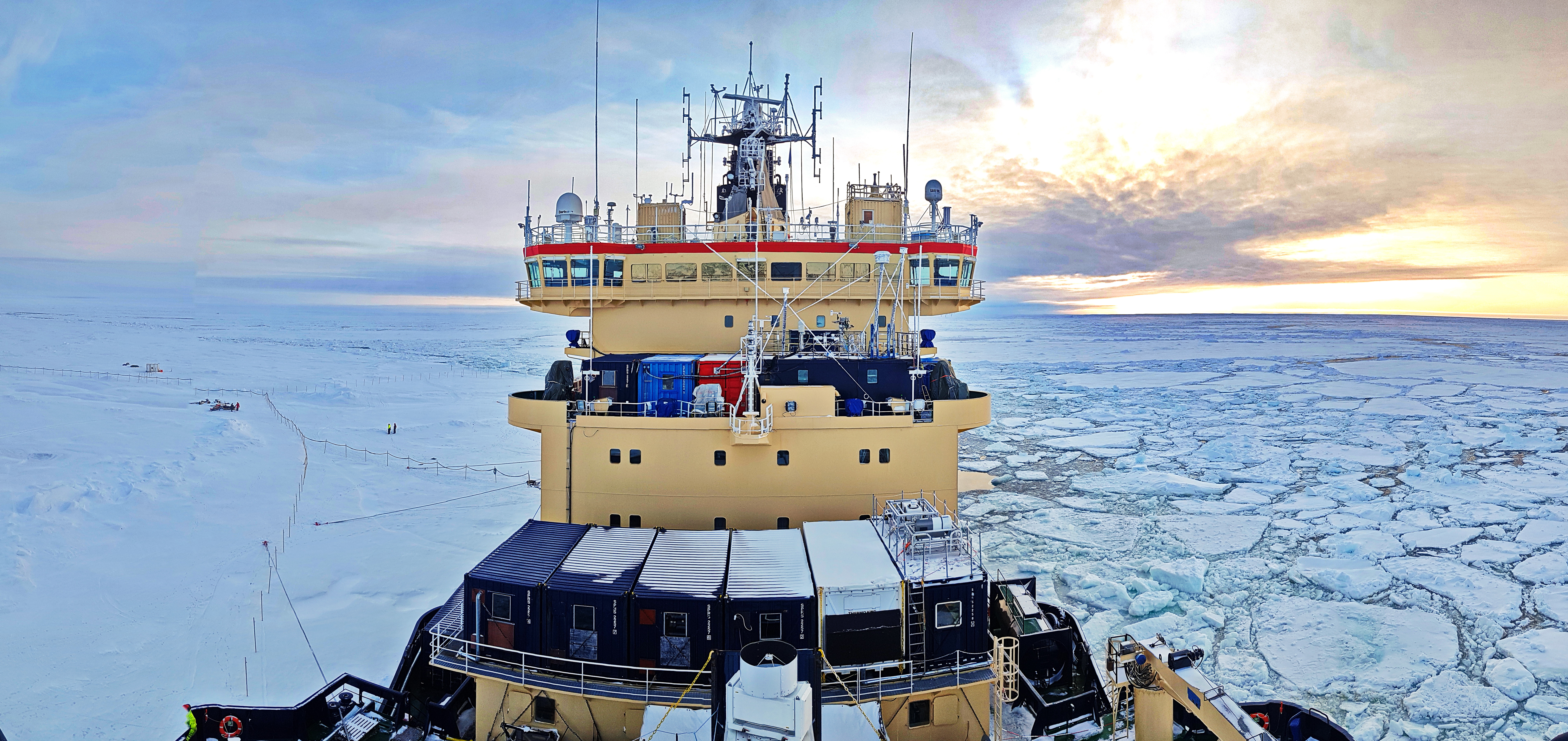
The primary purpose of on‑board weather forecasting was to support operational planning. In transit it was used for navigation, although the ship’s track was more dependent on ice conditions. Weather forecasts are crucial for determining when certain activities can happen, such as when to fly the helicopter, start deploying instruments on the ice or start packing up. For example, the ice camp operations were ended one day earlier than originally planned, a decision based on forecasts of an approaching storm. Work on the ice must always be planned with safety as the highest priority. It becomes dangerous in stormy conditions and in dense fog, when the polar bear guards on the ship’s bridge cannot see far enough to warn about approaching animals. But forecasts were also used for scientific decisions, for example on cloud top heights and wind speeds for the tethered balloon flights, or for when Oden had to be moved and rotated to keep the bow upwind to protect on‑board air-pollution sensitive instruments from contamination from the ship itself.

But weather forecasting for an icebreaker expedition to the high Arctic comes with some special challenges. Probably the most substantial is the limited communications bandwidth. The Internet is not available and therefore any forecast products had to be sent to the ship in a predetermined graphical format via a satellite phone email service, each message smaller than a few hundred kilobytes. Without the possibility to download any of the extra information provided from weather services as a part of the YOPP special observations periods, only limited predetermined data was available. A second challenge is that there are very few observations in the area other than our own, and on top of this the ship is moving. Even when moored to an ice floe, it moves, albeit slowly. So, the operational forecasting relied to a great deal on the experience of the ship’s forecast meteorologist, who on Oden also served as local air traffic controller for the helicopter operations, drawing on very limited numerical weather prediction output from ECMWF and real-time satellite imagery, received directly from polar-orbiting satellites. ECMWF data were used because national regional models do not cover the area in question.

ECMWF forecasts up to three days ahead were turned into tailored forecast maps at the Swedish Meteorological and Hydrological Institute (SMHI) and transferred via satellite phone link twice a day. One set of maps combined surface pressure, wind, precipitation and temperature and a second set of maps combined the 850 hPa geopotential, wind, temperature and relative humidity. The wind at about 140 m and vertically integrated lower-level precipitable water were provided on a third set of maps. APPLICATE collaborated with ACAS to provide an additional experimental forecast product for Oden’s position, twice daily. This was extracted from ECMWF’s operational high-resolution forecast (HRES) for a single column and was provided in the form of three graphical images, combining time–height sections of temperature and cloud water with 2-metre and skin temperature; a specific humidity time–height section with accumulated precipitation and cloud-water path; and a time–height section of wind speed with 10‑metre wind speed and direction. These were too large for the satellite phone email delivery and were transferred to Oden via satellite phone FTP.

Evaluating the forecasts

Important for understanding this evaluation is that both 3‑hourly SHIP observations and 6‑hourly BUFR messages from Oden’s soundings were assimilated in ECMWF’s Integrated Forecasting System (IFS). The forecasts were first evaluated subjectively by the ACAS Principal Investigator and the ship’s forecast meteorologist on the fly. The largest forecast challenge was clouds and fog, and here the IFS cloud forecasts provided little direct guidance. This was somewhat of a problem for AO2018 since low visibility prohibited work on the ice, due to polar bear hazards, and limited the use of the helicopter. However, quite often the predicted lower-troposphere precipitable water was more useful for judging the risk of fog than the cloud forecast directly from the model. In fact, this product was quickly nicknamed ‘fog chart’ even though there is neither visibility nor cloud water on the map. The failure to correctly forecast clouds also affected the surface energy budget and therefore the temperature forecast: predicted temperatures were often too high. The IFS wind forecast, on the other hand, quickly became considered very accurate, almost surprisingly so. Especially the wind direction forecast became trusted. This was important in AO2018 to determine when the ship had to be rotated to make sure the bow kept facing the wind, to limit contamination from the ship for some of the measurements.

The objective evaluation has now started, focusing on a few variables at first. We use observations from the 7th deck weather station, about 20 m above the surface, and 6-hourly soundings launched from Oden’s helipad, 14 m above the surface. For simplicity, we have interpolated IFS model output to the resolution of the sounding data. This results in a fine-scale vertical error structure that is meaningless and needs to be disregarded; the model does not have such a high vertical resolution and so could not be expected to resolve details in the soundings. We chose this method to avoid having to predetermine an appropriate averaging scale for the observations. For the 7th deck weather station, the observations were averaged over 5 minutes centered on the forecast time. We define model bias as the median difference between the model and observations.

As mentioned above, the IFS cloud forecast was a problem. The forecasts tended to overestimate cloudiness and did not capture the few cloud-free periods. The even fewer cloud-free periods that were predicted did not materialise in reality. One effect of this is clear in Figure 3, which shows overlapping 3‑day forecasts of 20‑metre temperature together with observations. For example, around 17 August the clouds dissipated and the observed temperature dropped for 2 to 3 days, down to –5°C, while the forecasts maintained the clouds and hence a too high temperature. It is interesting to note that the initial temperatures during this period were often lower, showing the effect of assimilating the observed temperature. However, the forecast warm bias returns within 6 to 12 hours. The predicted near-surface temperature features a pronounced warm bias throughout, which we believe is at least partly due to the cloud forecasts. Predicted temperatures are (almost) never below the observations and sometimes, during colder periods, the model is up to 6°C too warm. Before 28 August, when the surface is still melting, the predicted near‑surface temperature is near-constant at about 0.5°C. Although errors become larger later, this is an unphysical solution since the surface skin temperature of melting snow and ice cannot be above 0°C, even when the surface energy budget is constantly positive; all the surplus energy goes into melting and the temperature is stuck at the melting point. Preliminary data indicate that the net surface energy budget (not shown) is positive at about 20 W/m² until at least 23 August and does not go permanently below zero until around the end of August. Around 28 August, the predicted temperatures suddenly drop and then correctly stay below 0°C. While the warm bias in the forecasts actually increases when the surface energy budget becomes negative and the surface starts freezing, the forecasts faithfully capture the timing of rapid changes in temperature due to synoptic-scale weather.

Figure 4a reveals a distinct vertical structure of the bias in the temperature forecasts. It is interesting to note that, except at altitudes of about 0.5–1 km and 4–6 km, there is not much error growth with forecast length. The warm–cold–warm–cold bias structure with increasing altitude looks like a ‘model climate’ that the forecasts snap into very fast, even when provided with highly accurate initial conditions. Except in the boundary layer, the initial errors are small (Figure 4b). The boundary-layer error is large from the initial time and grows further over the first six hours, while in the 0.5–2 km layer a large negative bias develops, mostly over the first day. The largest errors thus appear in the layer below 2 km. The analysis so far indicates that the boundary-layer warm bias is related to the handling of the surface energy budget, which is probably also affected by cloud forecasts. The cold bias on top of the boundary layer is probably also due to errors in the prediction of clouds. Previous summer expedition data has indicated that the top of the very persistent low clouds is usually near the 1‑kilometer range. In other layers of the atmosphere, error growth is small and systematic errors are within a few tenths of a degree.

Outlook

We will continue to evaluate the IFS forecasts used during the expedition by looking at more variables, such as clouds and the terms in the surface energy budget, and also explore differences between forecasts initiated at 00 UTC and 12 UTC, to further analyse several of the features discussed above. Within APPLICATE we will also perform and evaluate forecast experiments with different new formulations. Work is already ongoing to address the issue of surface skin temperatures for melting snow and ice, to improve formulations of snow on the ice and for turbulent mixing in clouds. The data and evaluation from this observation campaign are being used by ECMWF to help identify shortcomings in the model physics. Progress in addressing the issues identified is already being made. This collaborative effort between ECMWF and the ACAS project thus illustrates the benefits of observation campaigns for model development. In June 2019, ECMWF held a workshop where leading scientists discussed how to further strengthen the many potential links between observation campaigns and model development.