As part of ECMWF’s continuous efforts to improve the representation of physical processes of the Earth system, an increasing number of km-scale simulations are performed. These activities are supported by the EU’s Destination Earth initiative (DestinE), in which ECMWF aims to create a high-resolution digital twin of our planet. Although higher-resolution simulations can improve the prediction of smaller-scale features and increase model fidelity, often the features’ exact location cannot be precisely determined. This results in traditional metrics such as root-mean-square error (RMSE) being degraded. Spatial verification techniques can provide a better indication of the value of such forecasts than traditional verification metrics by evaluating if the forecasts have the right statistics over a certain neighbourhood. Such techniques have been used in the limited-area modelling community for some time. In this article we describe how the Fractions Skill Score is being tested at ECMWF as a first step towards a more comprehensive evaluation of performance improvements at high resolution.
Verifying high-resolution forecasts
ECMWF’s current operational high-resolution global forecast (HRES) has a grid spacing of 9 km. Experimental forecasts with 4.5 km grid spacing are being generated as part of the first phase of DestinE, and even higher resolution runs have been performed in test mode. In order to evaluate the skill of surface fields at increasingly high resolution, methods beyond the standard point-wise matching of forecasts and observations need to be adopted. This is because of the so-called ‘double-penalty’ issue. A forecast predicting a feature with sharp gradients such as precipitation from a convective cell will be doubly penalised if it predicts the feature at a wrong space or time: once for missing the feature in the correct spot/at the right time, and once for the false alarm in the wrong place/at the wrong time (Figure 1). Hence the error will be twice as large as for a ‘flat’ forecast that does not predict the feature at all. Given the potential value of the forecast indicating the event, even if somewhat shifted, human judgement would consider the flat forecast as worse than the wrong-location/wrong-time forecast, especially if the displacement is small. The interpretation of gridded forecasts to issue warnings or assist decision-making typically relies on neighbourhood analyses rather than a literal interpretation of grid-point values. Double penalty issues are especially relevant for high-resolution fields with strong gradients and sharp features, such as precipitation or cloudiness.
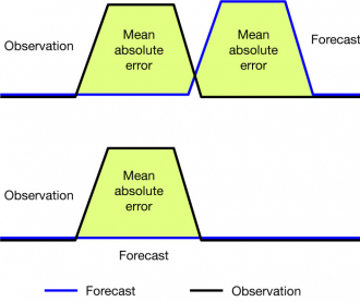
For a given level of imperfect association between forecasts and observations (a correlation coefficient smaller than 1), forecasts that minimise the point-wise RMSE have less variability than the observations. Therefore, a model with low variability (i.e. a lack of fidelity) will score better than a model with the right amount of variability. Based on the RMSE or related measures, it might be tempting to tune models towards lower variability. Hence, if physical realism of a model is sought, the RMSE may not be the proper metric to optimise.
One way of dealing with the double penalty issue is to compute scores for differently sized areas instead of just point-wise. A number of different spatial verification techniques have been developed (Brown et al., 2011). One of these, the Fractions Skill Score (FSS) introduced by Roberts and Lean (2008), has been widely used for the verification of limited-area model precipitation forecasts and is being tested at ECMWF as part of the move towards higher resolution. It gives a more complete picture of forecast performance for fields such as precipitation or cloudiness, since they may exhibit little skill at the grid scale but significant skill at larger scales. It also provides a natural framework for comparing forecasts at different resolutions, which is needed for km-scale model development and evaluation.
The Fractions Skill Score
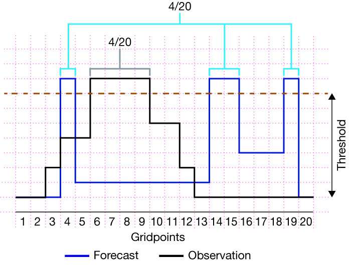
The FSS is a spatial verification technique that does not automatically penalise location errors such as the one depicted in Figure 1. It answers the question: did the observed feature occur in a nearby location in the forecast? To do so, it counts the fraction of grid points in a neighbourhood at which a given threshold (e.g. of precipitation amount) is exceeded, both in forecasts and in observations (Figure 2). Then it compares the two fractions by computing their squared difference. The neighbourhood analysis is done separately at each grid point and then averaged over the region of interest. The Fractions Skill Score is then obtained by normalising by the worst score that could be obtained from rearranging the forecast fractions field. Analysing multiple thresholds and neighbourhood scales makes it possible to get an idea of the spatial scales at which the statistics of the number of exceedances in the forecasts match the statistics of the observations. By constraining the statistics to a neighbourhood, the FSS requires some degree of association at larger scales, while allowing for smaller-scale location and shape errors.
Properties of the FSS
Like any verification metric, the FSS has some specific properties to be aware of. If the number of threshold exceedances in the forecast and observations are overall different due to imperfect calibration of a forecast, this will be penalised. It can be avoided by using quantile thresholds instead of absolute thresholds. Another property to note is that the FSS is not symmetric with respect to the definition of feature and non-feature. It will give different results depending on whether the grid points exceeding a threshold are counted or the ones below it. Finally, the FSS is not a traditional skill score that measures improvement over a fixed reference forecast, and although it ranges between 0 and 1, positive values do not automatically mean that the forecast is useful. According to Mittermaier & Roberts (2010) and Skok & Roberts (2016), a threshold of FSS = 0.5 may in most cases be a useful lower limit, although FSS values below 0.5 may still be regarded as useful for some applications if the forecasts are not perfectly calibrated.
Verification of HRES precipitation
Figure 3 shows the skill of daily-accumulated precipitation forecasts from the operational HRES over Europe (12.5°W–42.5°E and 35°N–60°N) for different thresholds in a winter and a summer month of 2019 (top and bottom rows, respectively). The observational dataset used for this evaluation is GPM-IMERG, which is a satellite-based, gauge-corrected gridded precipitation estimation. GPM-IMERG covers the latitudinal band between 60°S and 60°N and provides data every 30 minutes with a spatial resolution of 0.1 degrees. As a satellite-derived precipitation product, it has the advantage of providing high-resolution information across a large portion of the globe, while it shares the general weaknesses of satellite-derived estimates. Due to the indirect nature of the relationship between satellite measurements and precipitation amounts, both random and systematic errors are introduced. Gridded precipitation analyses based on rain gauges are more robust in this regard. However, they are typically available only at coarser resolution (0.25 to 0.5 degrees at most) and quite uneven in coverage. On the other hand, radar products provide information at very high resolution, but coverage is limited, and calibration procedures can be inhomogeneous across different countries’ networks.
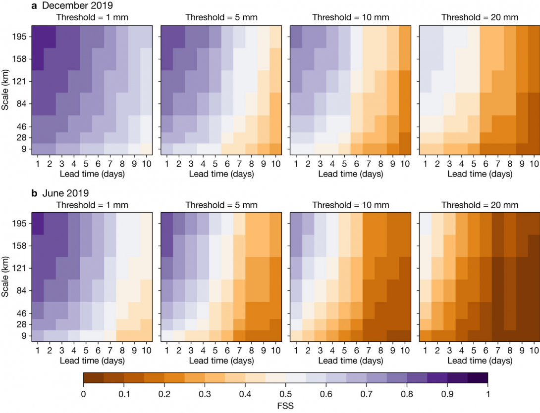
The 9 km HRES forecasts have been re-gridded to match the observations with a conservative interpolation method. Each panel in Figure 3 shows the FSS as a function of forecast lead time and neighbourhood scale from the grid-scale up to about 200 km. As expected, skill increases with scale at all lead times. Values above 0.5 (in purple) indicate that the forecast is useful at that scale. At a threshold of 1 mm in winter (leftmost panel of Figure 3a), the HRES is skilful for nearly all lead times and scales shown. In summer (leftmost panel of Figure 3b), forecast skill is lost after about 8 to 9 days, even at larger scales of 100 to 200 km. Moving to higher thresholds, the FSS generally decreases, so that at 20 mm some skill is left only in the short range and at large scales in winter, and little skill in summer. Generally, there is a substantial gain in skill when moving from the grid-scale to the next-bigger scale (boxes with 3x3 grid points).
Using a threshold of FSS = 0.5 to determine the usefulness of a forecast is strictly applicable only if the forecast and observation datasets are unbiased. As this is not the case, even FSS values below 0.5 may be useful and provide better-than-random guidance on the spatial precipitation distribution.
Verifying radiation with the FSS
A useful proxy for the verification of cloud macro-properties, such as total cloud cover and cloud optical depth, is the downward shortwave radiation flux at the surface. Like precipitation, it is a flux quantity that can exhibit strong gradients and high variability in space and time, and it can be estimated using satellite observations. Figure 4 shows how the operational HRES forecast skill for this quantity varies with spatial scale and lead time in the summer season in the domain 60°W–60°E and 60°S–60°N. The verification dataset used is EUMETSAT’s Climate Monitoring Satellite Application Facility (CM SAF) 24-hour average of downward shortwave radiation at the surface. A threshold of 200 W/m2 has been found suitable for the domain during summer. The FSS is not sensitive to the exact value of this threshold as long as it separates predominantly clear and cloudy areas.
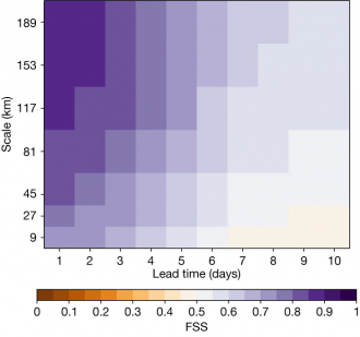
In terms of absolute FSS, we can see similar values (0.85 to 0.9) at large scales and short lead times as for summer precipitation with a low threshold of 1 mm (shown in Figure 3b). As for precipitation, skill becomes small beyond forecast days 7 to 8, and this limiting lead time is not very sensitive to scale.
Evaluating brightness temperature for case studies
The Fractions Skill Score is also useful for evaluating individual cases, such as the ones currently being investigated in the Extremes Digital Twin of DestinE. The FSS makes it possible to compare the performance of different model configurations during specific events that were relevant to society due to their impacts. This type of individual case study analysis does not replace a statistical verification over longer periods but can uncover weaknesses which are difficult to detect in statistical performance summaries.
The left-hand panel in Figure 5 is a satellite image showing cloudiness during storm Ciara that affected western Europe between 7 and 9 February 2020. A large-scale synoptic trough over the North Atlantic has a clearly developed frontal cloud. The grey scale indicates brightness temperature from the infrared window band of 10.8 µm. Light colours can be used as a proxy for cloud top height, while darker colours indicate surface temperatures under clear-sky conditions. The central and right panels show simulated satellite images derived from experimental ECMWF forecasts at 9 and 4.5 km with a lead time of 48 hours. In the blue domain, a region of cold air advection, the 4.5 km experiment produces smaller-scale clouds than the 9 km run, which are prone to double-penalty issues. In the orange domain, the frontal system is wider in the 4.5 km experiment than in the 9 km run. Both experiments underpredict a narrow band of lower clouds to the southeast of the front.
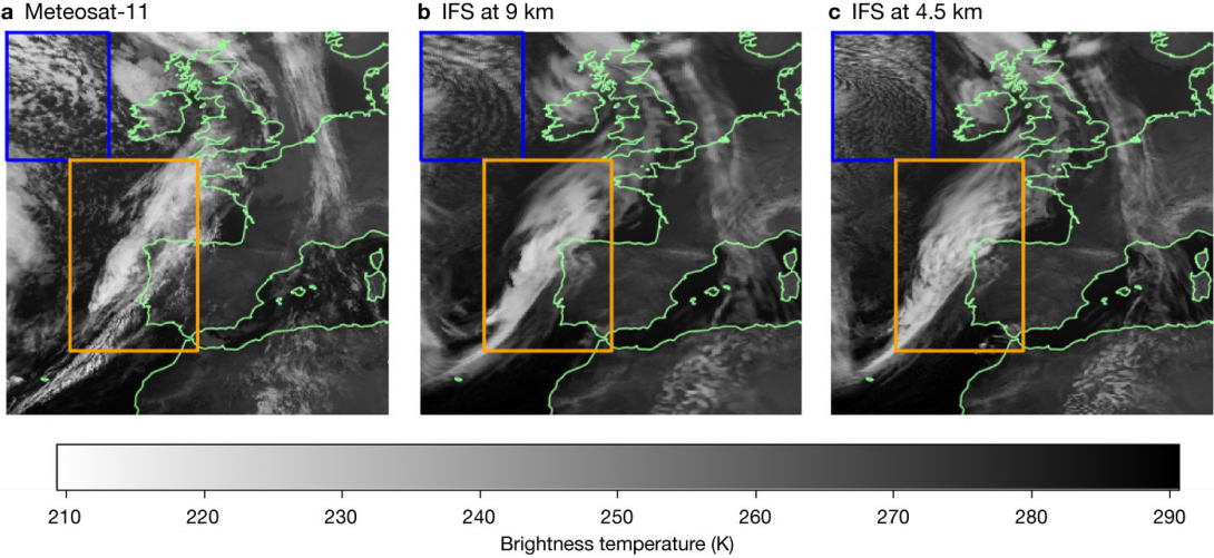
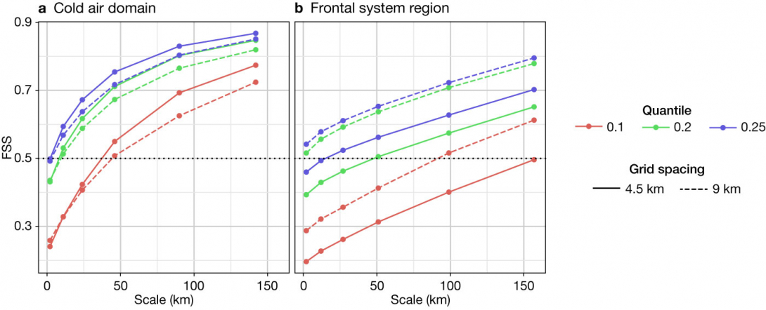
Figure 6 compares the FSS of the 9 and 4.5 km experiments for the two selected regions. As these simulated satellite images are known to have a warm bias, the FSS has been computed for quantiles instead of absolute thresholds. These quantiles are derived from the distribution of brightness temperatures within the selected domains. For the cold air region, we can see that the FSS is below 0.5 at grid scale, and there are no clear differences between the two runs. However, when looking at larger scales, the 4.5 km run produces better agreement with the observations for all quantiles, becoming useful already at a neighbourhood size of 5x5 grid points for quantiles 0.2 and 0.25. For the frontal region the situation is reversed: the 9 km experiment performs better than the 4.5 km one at all scales and for all chosen quantiles. In the 4.5 km run, the front is too wide when compared to observations, and this large-scale error is only compensated in the FSS when evaluating rather large neighbourhoods. This single case serves to illustrate how the relative skill in predicting cloud systems between runs at different grid spacings can vary strongly with the type of system. A more systematic evaluation of the FSS for different cloud regimes will help identify possible causes of such differences.
Outlook
The method described here to evaluate forecasts with a scale-dependent metric as an additional verification measure will be important in the future as model resolution increases. Spatial verification techniques have been developed and used for some time within the limited-area modelling community, such as in ECMWF’s Member and Co-operating States, and ECMWF is benefiting from these efforts. Although those techniques are well established, new developments that simplify and facilitate the interpretation of verification results are still taking place (e.g. Skok, 2022). Another essential aspect to be improved is the availability of high-resolution, high-quality observational datasets with wide coverage for verification. There is a need to understand the associated uncertainties and potential biases of existing observational datasets used in verification. For precipitation in particular, it will be important to compare different gridded verification datasets to assess their respective strengths and weaknesses. Scale-dependent metrics are relevant for other highly variable fields, such as clouds, and infrared and visible satellite images can be used to verify cloudiness as a function of scale. Computation of the FSS or similar scores will therefore be part of future evaluations of operational changes for the HRES as well as ensemble forecasts (ENS), and it will help to provide a more complete picture of the performance of new model cycles.
Acknowledgement
This contribution has been produced with support from the Destination Earth initiative and relates to tasks entrusted by the European Union to ECMWF, which is implementing part of this initiative funded by the European Union.
Further reading
Brown, B.G., E. Gilleland, & E.E. Ebert, 2011: Forecasts of Spatial Fields. In Jollife, I.T., D.B. Stephenson (editors), Forecast Verification, Wiley, 95–117. Doi:10.1002/9781119960003.ch6
Mittermaier, M. & N. Roberts, 2010: Intercomparison of Spatial Forecast Verification Methods: Identifying Skillful Spatial Scales Using the Fractions Skill Score, Weather and Forecasting, 25(1), 343–354. Doi:10.1175/2009waf2222260.1
Roberts, N.M. & H.W. Lean, 2008: Scale-Selective Verification of Rainfall Accumulations from High-Resolution Forecasts of Convective Events. Monthly Weather Review, 136(1), 78–97. Doi:10.1175/2007mwr2123.1
Skok, G. & N. Roberts, 2016: Analysis of Fractions Skill Score properties for random precipitation fields and ECMWF forecasts. Quarterly Journal of the Royal Meteorological Society, 142(700), 2599–2610. Doi:10.1002/qj.2849
Skok, G., 2022: A New Spatial Distance Metric for Verification of Precipitation. Applied Sciences, 12(8), 4048. Doi:10.3390/ app12084048