
ECMWF assimilates a wide range of observations to help define the initial conditions at the start of a forecast run. It uses a complex data assimilation scheme (4DVAR) to make the best possible use of the available observations. Given the importance of accurate initial conditions for the quality of forecasts, it is useful to monitor and understand the relative impacts of different parts of the observing system on the analysis as well as on forecasts. ECMWF routinely assesses Forecast Sensitivity to Observation Impact (FSOI) using an ‘adjoint-based’ approach where forecast skill is evaluated with respect to analyses. An alternative, observation-based measure of impact called ‘observation-minus-forecast (OMF) residuals’ has been implemented and found to provide complementary results. Results using the OMF residuals approach differ from FSOI but confirm the strong influence of satellite observations, which dominate the observing system in terms of volume. Both measures show that in-situ measurements remain an essential component of the observing system despite their relatively low numbers compared to satellite observations.
The overall impact of observations on the analysis and on forecasts depends on the quality of the assimilation system and the forecasting model and locally on the characteristics of the Earth’s surface and dominant weather regimes. The relative impact of each component of the observing system depends on its quality, spatial and temporal distribution, prescribed observation errors (derived from a long-term statistical evaluation of the observing system) and inherent redundancies with other components of the observing system. To estimate the impact of observations, different methods are used. The results obtained depend on the verification measures employed and the atmospheric structures targeted.
Observation impact methods
Data denial experiments (generally referred to as Observing System Experiments or OSEs) are the most appropriate method to quantify the impact of individual components of the observing system. They are systematically performed before actively assimilating new observation types. Occasionally data denial experiments are conducted to help ECMWF and data providers optimise the assimilation system or to give valuable information about current observing systems and guidance for future observing systems. However, OSEs are expensive because they necessitate additional long-term data assimilation and forecast experiments, denying each observing system under investigation one by one. This cannot be done frequently to evaluate the many different components of the observing system. OSEs are therefore not suitable for day-to-day monitoring. Efficient and less expensive complementary tools have been developed for that purpose.
So-called ‘adjoint-based’ approaches offer a powerful complement to OSEs by estimating the contribution of different types of observations to the increase or decrease in forecast error. These methods identify the relationship between the short-range forecast error (evaluated against the analysis) and the observations used in the assimilation (Box A). An adjoint-based FSOI system was implemented operationally at ECMWF in June 2012 and is run every day to continually produce estimates of observation impact (Cardinali, 2009).
Todling (2012) suggested another approach to estimate observation impact by making use of differences between observation-minus-forecast residuals (OMF residuals) obtained from consecutive forecasts (Box B). This approach is simpler and less costly than FSOI but it assumes a high degree of temporal homogeneity in the observing system. Liu & Kalnay (2008) have proposed an ensemble-based observation impact estimation technique that does not require the use of forecast model and data assimilation adjoints. This approach is not discussed in this article but will be explored in the future, using the EDA (Ensemble of Data Assimilations).
Limitations
Observation impact methods are based on assumptions and approximations that need to be taken into account when interpreting the results. The main considerations for the adjoint-based approach using the analysis as the verification state are that:
- Errors in the analysis can mask the impact of observations. In extreme cases, such errors are incorrectly interpreted as a negative impact of observations.
- The verification state should ideally be uncorrelated with the forecast. This is not the case when the analysis is used.
- Different choices of forecast error measure (the ‘norm’) can be made and this fundamentally affects the resulting estimates of observation impact.
- The adjoint-based method is restricted by the use of a linearised version of the model, which makes it valid only to evaluate short-range forecasts (0 to 48 hours).
- Biases in the model (compared to the analysis) may erroneously be interpreted as a negative impact of observations, where they really represent model errors.
The main considerations for OMF residuals are that:
- The method captures only part of the forecast error (the part projected onto the space of observations) and the choice of norm is very limited.
- The method assumes sufficient homogeneity of the observing system between the initial time and the verification time. Such an assumption means that any conclusions regarding observation impact should be based on statistics and cannot be applied to individual cases or individual stations.
- Since some observations are bias-corrected, there is an undesirable correlation between the forecast and the verification.
Observation impact results

|
AIRS |
Atmospheric Infrared Sounder |
|
IASI |
Infrared Atmospheric Sounding Interferometer |
|
CRIS |
Cross-track Infrared Sounder |
|
AMSU-A |
Advanced Microwave Sounding Unit-A |
|
ATMS |
Advanced Technology Microwave Sounder |
|
MHS |
Microwave Humidity Sounder |
|
SSMIS |
Special Sensor Microwave |
|
AMSR2 |
Advanced Microwave Scanning Radiometer 2 |
|
GMI |
Global Precipitation Measurement (GPM) Microwave Imager |
|
MWHS2 |
MicroWave Humidity Sounder 2 |
|
SATOB |
Atmospheric motion vectors |
|
SCATT |
Scatterometer |
|
GEOS |
Geostationary Operational |
|
GPSRO |
GPS radio occultation |
|
TEMP |
Radiosondes |
|
AIREP |
Aircraft reports |
|
ACARS |
Aircraft Communications |
|
AMDAR |
Aircraft Meteorological Data Relay |
|
SYNOP |
SYNOP network weather stations |
|
DRIBU |
Buoys |
|
METAR |
Weather reports from airports |
|
PILOT |
Wind observations from PILOT radiosondes and radar profilers |
|
SHIP |
Ship-based instruments |
|
MWHS |
MicroWave Humidity Sounder |
Table 1 Components of the global observing system.
Adjoint-based observation impact technique
Langland & Baker (2004) introduced an adjoint-based approach to estimate the impact of observations on short-range forecasts (the adjoint is a matrix transpose which back-projects information from data to the underlying model). In the adjoint-based approach, a forecast error measure is defined involving the comparison of the forecasts against a proxy of the true state. The change in this error measure, computed for forecasts valid at the same time issued from two consecutive analyses, is solely due to the assimilated observations. Using the adjoint of the model and the analysis, one can relate the change in the forecast error to assimilated observations. The forecast error measure ef is defined as:
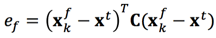
Where xkf and xt are the predicted (from initial time k) and true states, respectively. C is a weight applied to the forecast error. Consider forecasts from the analysis xa and the background xb, which is a short-range forecast based on the previous analysis. The difference δef = ef(a) – ef(b) measures the combined impact of all observations assimilated. It can be estimated as a sum of contributions from individual observations using information from the model and analysis adjoints. Approximations of the variation in e due to variations in xa and xb are given by the Taylor series with various orders of approximation. The second order approximation used in the ECMWF FSOI implementation (Cardinali, 2009) is:

where y is the observation vector, h is the observation operator transforming model values into observation-like values, KT is the adjoint of the analysis, and MaT and MbT are the matrices of the model adjoint based on trajectories starting from the analysis and the background, respectively. For any set of observations, δe < 0 represents a reduction in forecast error. δe > 0 means that the observations have caused an increase in forecast error.
Since the true state is unknown, the method uses the analysis or observations as a proxy of the truth. In the ECMWF implementation, the analysis is used. The error measure is computed globally and weighted using a dry energy norm. Other choices of the weight (norm) might lead to a different estimation of the impact (Todling, 2012) and therefore it is important to take this into account when interpreting impact results. The dry energy norm used at ECMWF gives more weight to tropospheric observations. With this method other bespoke norms can be adopted.
When observations are used as a proxy of the truth, the weight is the observation errors as used in 4DVAR. This variant of the adjoint-based approach has been tested at ECMWF but not yet implemented.

Schematic of forecast error measure. Adapted from Langland & Baker (2004).
In order to compare the results from OMF residuals and adjoint-based approaches, we accumulated statistics for a three-week period. For the adjoint-based approach, we used operationally produced FSOI statistics (based on IFS Cycle 43r1, operational since November 2016). Statistics from the OMF residuals approach were derived from an experiment run at the operational resolution (IFS Cycle 43r1). Figure 1 shows the relative 24-hour observation impact per data type derived from the operational adjoint-based approach and the OMF residuals. Statistics cover the period from 6 to 28 November 2016. ACARS (Aircraft Communications Addressing and Reporting System) data have greater impact according to the OMF residuals method than they do according to the adjoint-based approach, likely because reduced impact from data redundancy for dense aircraft data over the USA is handled better by FSOI. The two hyper-spectral instruments CrIS and IASI appear to have more estimated impact using the OMF residuals method. For these two instruments overcast observations (completely cloudy scenes) are used in the analysis. In a small number of cases the forecast departures have very large negative values, which indicates a significant mismatch of cloudiness between the forecast and these overcast pixels. When these cases are detected the inter-channel correlation of observation errors are partially ignored in the computation of observation impact to avoid affecting the results for other channels. GPS radio occultation (GPSRO), atmospheric motion vectors (SATOB), scatterometers (SCATT), radiosondes (TEMP) and buoys (DRIBU) appear to have less impact according to the OMF residual measure. Due to a temporary outage of data from two key satellites (Metop-B and AQUA), the impact of AMSU-A (Advanced Microwave Sounding Unit-A) satellite data is less important here than in previously documented results (Cardinali, 2009). As indicated by the small standard deviation bars in the data count (Figure 2), the observing system was stable throughout the period, which is important for the validity of results from the OMF residuals approach.


The differences between the two measures of impact are related to the nature of the forecast error measure (the applied norm, see Box A). The forecast error measure in the adjoint-based approach using the analysis for verification is more encompassing as it is computed in model space involving all grid points. In the OMF residuals approach the forecast error measure is computed against available observations, which means that non-observed parts of the atmosphere are not captured. The total dry energy norm applied in the adjoint-based approach has more weight in the troposphere and the lower stratosphere than the norm used in the OMF residuals approach. In the latter, the weight is based on observation errors used in the assimilation system. They are more uniform with height. The impact of the norm is clearly visible when comparing the relative impacts of observations per vertical level, as shown in Figure 3 (for AMSU-A) and Figure 4 (for GPSRO). Here the impact for stratospheric observations is greater according to the OMF residuals measure than it is for the adjoint-based measure, and it is significantly smaller for tropospheric data. Looking at the average impact per individual observation (Figure 5), it is clear from both measures that in-situ observations have a greater impact per observation. Buoys, ships, SYNOP weather stations and AIREP aircraft reports have the greatest impact per observation. The average impact of buoys is the highest, but according to the OMF residuals method it is not significantly bigger than that of SYNOP reports. Impact results obtained using the OMF residuals approach are in agreement with previous results obtained at ECMWF using an alternative implementation of the adjoint-based method (verified against observations and weighted by observation errors).
Observations impact using OMF residuals
Todling (2012) suggested a simpler and cheaper approach compared to FSOI for assessing observation impact using OMF residuals. The forecast error measure is computed using observations as a proxy of the truth. It is expressed as:
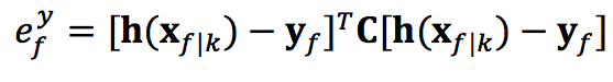
where h denotes the observation operator, xf |k the forecast valid at the time f and issued from time k, yf represents verification observations at the time f, and C is the inverse of the observation error variance. Similar to the adjoint-based approach, the forecast error reduction is determined by computing the difference between the error measures for forecasts valid at the same time issued from two consecutive analyses:
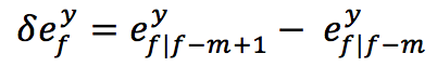
where m is the forecast range.
The approach is based on the assumption that the observing system is sufficiently homogenous between the initial time and the verification time for the partitioning of the impact into individual contributions from the various components of the observing system to be done at the verification time. Such an assumption is believed to allow a good projection (in a statistical sense) between the forecast error measure (computed by construction against observations at verification time) and the set of initial observations used. For this assumption to work the computation of the forecast error measure should involve only observations selected for use in the data assimilation (and not all available observations). Since the approach does not explicitly involve using the model adjoint, it can be applied to forecast ranges beyond the validity range of the model tangent linear. Applying the approach to step zero provides the impact of observations on the analysis. Observation impact results (fractional contribution) computed for the 24-hour forecast range can be compared to the operational adjoint-based FSOI.
OMF residuals are going to be computed routinely for all observations used operationally at ECMWF.
Discussion
Adjoint-based approaches are well established to estimate the impact of observations on forecasts. Their main limitation is related to the verification state. When used as a reference, both the analysis and observations have limitations and it is advantageous to use both and to compare the results. ECMWF runs operationally an adjoint-based method using the analysis as the verification state. It is expected that in the near future the Centre will begin to routinely compute forecast departures in observation space to be used for verification. The availability of such forecast departures will make it easy and virtually cost-free to estimate observation impact in observation space. At least for short-range forecasts, the OMF residuals approach seems to provide sensible results that will complement the routinely produced FSOI statistics. The complementarity of the two approaches is mainly explained by their use of different verification references and choices of weight assigned to the forecast error measure.
Summary and prospects
For many years, ECMWF has been using an adjoint-based approach to estimate the impact of observations on forecasts. Although the method provides good guidance on the impact of observations, diagnostic activities will benefit from having access to complementary impact results based on observations as a proxy of the truth, and also using another error norm. The expected availability of observation-minus-forecast (OMF) residuals will enable the routine, virtually cost-free computation of such additional diagnostics. The OMF residuals approach has the potential to be used for the estimation of observations impact at longer forecast ranges. This will be explored further and the results will be evaluated using the estimated impact of observations based on Observing System Experiments.
Further Reading
Cardinali, C., 2009: Monitoring the observation impact on the short-range forecast. Q. J. R. Meteorol. Soc., 135, 239–250.
Dahoui, M., G. Radnoti, S. Healy, L. Isaksen & T. Haiden, 2016: Use of forecast departures in verification against observations. ECMWF Newsletter No. 149, 30–33.
Langland, R. H. & N. Baker, 2004: Estimation of observation impact using the NRL atmospheric variational data assimilation adjoint system. Tellus, 56A, 189–201.
Liu, J. & E. Kalnay, 2008: Estimating observation impact without adjoint model in an ensemble Kalman filter. Q. J. R. Meteorol. Soc., 134, 1327–1335.
Todling, R., 2012: Comparing two approaches for assessing observations impact. Monthly Weather Review, 141, 1484–1505.
doi:10.21957/51j3sa