Visualising ML-based forecasts
The AIFS, the ML model developed at ECMWF, is run experimentally in a deterministic and an ensemble version. As open data, the deterministic AIFS forecast is available 4 times daily, out to 15 days. Also, both deterministic and ensemble products for the AIFS can be visualised on our website. With the engagement of the weather forecasting community, we aim to learn how these new models behave and perform in various situations, from various standpoints.
ML models developed by other institutions are also run routinely at ECMWF, initialised with IFS analysis, and made available for visualisation. Again, the goal is to learn about ML-based forecast performance and characteristics, from a variety of models of this new type. Besides ECMWF’s own AIFS, the open charts catalogue comprises the following models so far: Pangu-Weather (Huawei), GraphCast (Google DeepMind), and FourCastNet (Nvidia). FuXi (Fudan University, Shanghai) was included until recently, but we have recently decommissioned that model and have welcomed a new entry.
The new entry in the open charts catalogue is Aurora, a model developed by Microsoft Research. Aurora is trained not only on ERA5 reanalysis data (the fifth-generation ECMWF atmospheric reanalysis, produced by the Copernicus Climate Change Service) but also on other datasets, including CMIP6 climate model experiments and NOAA’s GFS forecasts. Another key difference between Aurora and the other ML models run routinely at ECMWF is its spatial resolution. The version of Aurora that we run has a spatial resolution of 0.1° (~11 km), while the others are on a 0.25° grid (~28 km).
Forecast realism
Before entering ECMWF’s experimental forecast catalogue, forecasts based on new ML models are scrutinised. Among other statistical characteristics, a form of forecast realism is assessed using power spectra. Power spectra show the level of energy in the forecast at different scales, a way to diagnose the forecast ‘structural’ realism.
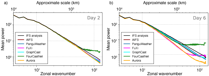
As an example, power spectra of geopotential height at 500 hPa for various forecast lead times are shown in Figure 1. By comparing results at day 2 (a) and day 6 (b), we see how Aurora and FuXi tend to lose energy at smaller scales at longer lead times, while this feature is less marked in the other ML models’ spectra. We also note that FourCastNet, here in its v2-small version, unphysically gains energy at small scales with the forecast lead time. Deviations by ML models from the true spectra of the atmosphere may impact the value of these systems to particular use cases.

Figure 1: Power spectra of IFS analysis and ML-based forecasts for geopotential at 500 hPa at a) day 2 and b) day 6.
The accuracy–activity trade-off
Forecasts with low energy at smaller scales appear visually smooth. This characteristic can lead to good scores, but forecast smoothness is sometimes undesirable from the forecast user perspective. The trade-off between activity and accuracy when generating forecasts with ML models has been discussed in a previous blog post.
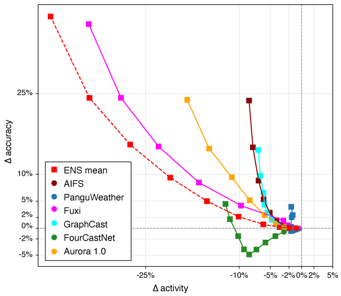
A holistic view of these two forecast attributes is provided by showing forecast accuracy versus forecast activity, in relative terms, on the same plot. Figure 2 illustrates how activity and accuracy jointly vary for successive forecast lead times. Ideally, a forecast would have an activity close to the activity of the analysis (for Δ activity, the closer to 0 the better) and, at the same time, improved scores with respect to the IFS control forecast (for Δ accuracy, the higher the better).

Figure 2: Forecast accuracy–activity trade-off for geopotential height at 500 hPa over the northern extratropics. The plot shows the forecast relative accuracy with respect to the IFS control forecast versus the forecast relative activity with respect to the IFS analysis. Results for forecasts at lead time day 1 (dot) up to day 10 (squares) are plotted. Accuracy is here measured with the anomaly correlation coefficient.
All ML-based forecasts present less activity than the IFS analysis but tend to have better scores than the IFS control forecast, here in terms of anomaly correlation, especially at longer lead times. These forecasts also tend generally to behave differently than the IFS ensemble mean, which by design washes out unpredictable features in the forecast.
One exception is Fuxi, which has similar attributes to the ensemble mean after day 5 with a large gain in accuracy at the expense of a large reduction of the forecast activity.
Because of this resemblance with the ensemble mean in the medium range, it was decided to decommission FuXi from our charts catalogue. In our view, delivering something like the ensemble mean has limited value for users. Users who wish to examine FuXi themselves can continue to do so, thanks to the recent ability for users to run these models from ECMWF’s open-data stream.
For the AIFS, accuracy and activity appear balanced differently with a substantial accuracy gain but, at the same time, a forecast activity that does not drift with the forecast lead time. We still see room for improvement in the AIFS and will be aiming to improve both activity and skill with future cycles. For Aurora, the forecast attributes are within the bulk of accuracy/activity observed with the other ML models.
Surface scores and spatial resolution
Verification against observation measurements is complementary to scores computed using IFS analysis as a reference, as in the example above. When using surface observations for verification, one assesses the forecast for quantities usually more relevant to the users. For example, 2 m temperature could be more useful than temperature at 850 hPa for some applications.
However, one should keep in mind that the output of NWP or ML models is a grid-box average, not a forecast at a specific point. The unfairness of a direct comparison of a model output with a point measurement is known as the representativeness issue in verification.
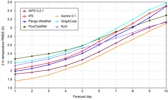
An example of verification scores for surface variables is shown in Figure 3. The root-mean-square error (RMSE) is plotted as a function of the forecast lead time for the different ML models present in our catalogue and compared here with the IFS operational forecast.
In this example, the AIFS performs comparatively well against Aurora, which is showing the best score for 2 m temperature. The spatial resolution of the models plays a crucial role here. Indeed, the Aurora spatial grid resolution is 0.1° (~11 km), similar to the resolution of the current IFS model, while the spatial resolution of the other ML models is 0.25° (~28 km).
For the AIFS team, this is a good motivation to reach this higher resolution, which we target for 2025.

Figure 3: RMSE of 2 m temperature forecast over Europe (June, July, August 2024) as a function of the forecast lead time.
A more comprehensive set of scores available
Verification of surface variables against observation measurements is now also part of our publicly available open data as well as in ecCharts for licensed users. Along with verification of upper-air variables (geopotential height at 500 hPa and temperature at 850 hPa), scores for 2 m temperature and 10 m wind speed are shown on the web to help monitor ML model performance.
Another new feature in the catalogue are scores displayed in the form of time series for selected variables. Performance for every day of a season can be plotted for pre-defined geographical areas. These time-series illustrate the day-to-day variability of scores, and how performance varies for different predictability regimes, consistently or not among ML models and the IFS.
Scores are updated on a three-month basis, at the turn of a new season, to show the performance over the season that just finished. Results for Aurora will be included in the next scores update on our website.