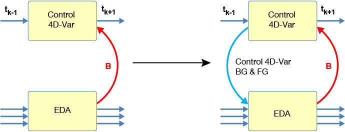
The Ensemble of Data Assimilations (EDA) will in Cycle 48r1 of the Integrated Forecasting System (IFS) change to a more accurate and computationally efficient configuration we call a ‘soft re-centring EDA’. In this new configuration, the EDA is approximately 30% cheaper to run than the current EDA for the same resolution. This computational saving will make the increase in resolution of the EDA also planned for Cycle 48r1 affordable.
Soft re-centring to improve analysis accuracy
In the EDA, we have an ensemble of perturbed members that are used to prepare a background error covariance matrix B for the next analysis cycle and that are also part of the initial conditions of ensemble forecasts (ENS). In addition, the EDA has an unperturbed control analysis that provides some information to perturbed members’ analyses, such as observation bias correction and ‘pre-conditioning’ information that speeds up a perturbed member’s analysis.
Re-centring is a commonly used technique in ensemble assimilation and forecasting. It regards ensemble members as perturbations from their mean, which are added to a more accurate re-centring state as a post-processing step. This improves the accuracy of the ensemble. We do this when initialising ENS from EDA forecast perturbations added to the latest available high-resolution 4D‑Var analysis. We have so far not used re-centring in the EDA itself to improve the analysis of perturbed members. However, when we looked in detail, we found that we could improve the starting state of the perturbed members’ analyses by incorporating information from a more accurate control analysis.
The ‘soft re-centring’ concept comes from incorporating information from the control member as input to a perturbed member’s analysis, rather than taking a perturbed member’s output and re-centring it on the control member’s analysis (‘hard re-centring’). In a soft re-centring EDA, the control analysis thus becomes part of the cycling of the perturbed members’ analyses (see the figure). In soft re-centring, the control member’s analysis is run in a 4D‑Var configuration with three 9 km outer loops with 50 km/50 km/40 km minimisations, closer to the high-resolution (HRES) 4D‑Var. The gain in accuracy makes it possible to run perturbed members with a cheaper 4D‑Var configuration with only one 9 km outer loop with 40 km minimisation, without loss of overall accuracy. Additionally, the fact that the re-centring is done inside the 4D‑Var minimisation helps to significantly reduce initial imbalances.

How does soft re-centring integrate the control member analysis? After the first minimisation of the control member has finished, the perturbed members’ analyses start, incorporating the additional information from the control’s preliminary analysis. First, the difference between control and ensemble mean background state is added to the background of all perturbed members, re-centring the perturbed members on the control background. This step improves the accuracy of the EDA mean analysis. The second step is to add the control member preliminary analysis increment to the perturbed members’ re-centred background to give a first guess trajectory that on average moves each member’s first guess closer to the final analysis solution. This second step is analogous to what we already do in the continuous long-window data assimilation (Co‑LWDA) introduced in the HRES 4D‑Var in IFS Cycle 47r1 (see the article by Hólm et al. in ECMWF Newsletter No. 163), where the early-delivery analysis is used as first guess in LWDA. In summary, the control member shows the perturbed members’ analyses how on average to account for new observations, and soft re-centring includes this average information as a starting point for the perturbed members’ analyses. The new control is not just an unperturbed member of the EDA as previously, but effectively an HRES clone (though not yet in real time), and it paves the way for a future tighter coupling of HRES 4D‑Var and the EDA.
Effect on forecast performance
In terms of forecast performance, the soft re‑centring EDA brings a small but visible improvement in the EDA control. This comes from more consistent estimates of the background error covariance matrix B. There are large improvements in the forecast skill of individual EDA members and an increase in spread of the whole EDA, which are visible when we start an ENS forecast directly from the EDA initial conditions. Some of these improvements remain visible also in the operational-like ENS setup, where 6‑hour EDA forecasts are hard re-centred on the control analysis and singular vectors are also added.