In the summer of 2023, ECMWF set about creating a data-driven forecasting system. From the outset the mindset has been for probabilistic prediction. Probabilistic prediction, typically achieved for physics-based models via ensemble forecasts, is central to ECMWF’s strategy. So even if the first version of the AIFS was a deterministic model, this has been viewed as a stepping stone to probabilistic prediction.
Now, one year on, we make the next step on that journey by introducing a first probabilistic version of the AIFS. We are making this model available very early in the development process, in no small part because of the fantastic engagement we’ve seen from the meteorological community exploring the AIFS and other data-driven weather forecasts, for instance through social media posts on snowstorm and heatwave forecasts. Seeing the community discover the current strengths and weaknesses has been very useful as we collectively develop a new way of making medium-range weather forecasts.

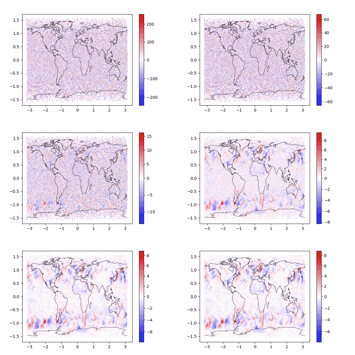
Figure 1: Illustration of how the model produces a forecast tendency (for meridional wind at 850 hPa) starting from random noise when provided with the previous atmospheric state.
How does this version of the ensemble AIFS work?
Like the excellent work from the GenCast team, we have followed the design principles set out by Karas et al. on how to build diffusion-based models, a generative AI method which is very popular in the context of image and video generation (see Jascha Sohl-Dickstein et al. and Jonathan Ho et al.).
For weather prediction, forecasting is formulated as a de-noising task. This means that in training, the neural network learns to remove noise from a future atmospheric state (technically a forecast tendency), conditioned on the current state of the atmosphere. When the model then produces a forecast, the task of making a prediction for the next timestep (for us here 12 hours presently) is broken down into a series of substeps (see Figure 1).
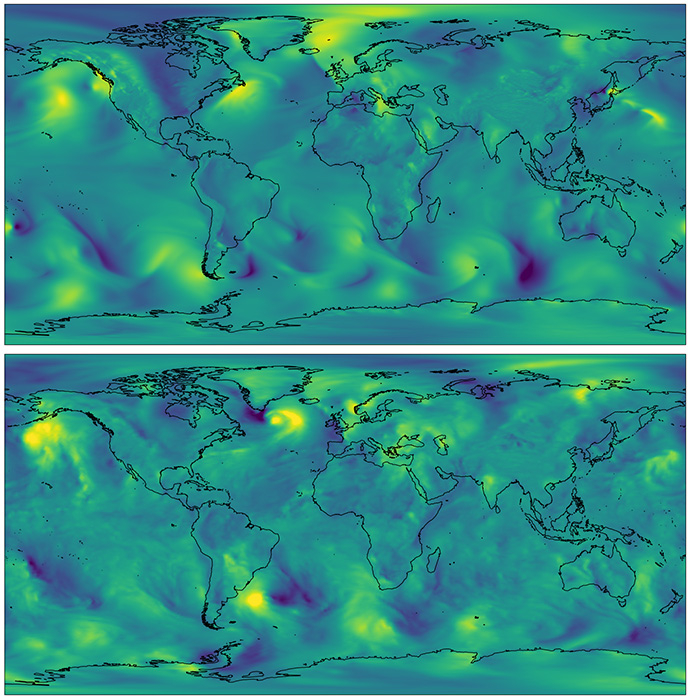
At the start of this process, the model is provided with the conditioning, i.e. the state of the atmosphere at present, and random noise. Then, over these substeps, the model iteratively removes noise, producing a noise-free prediction. This process is then repeated for the next timestep. Framing the problem in this way is inherently probabilistic: for a given current state of the atmosphere, the model can be called many times starting from different random noise fields to provide an ensemble of predictions for the next state, capturing the uncertainty of the forecast. Importantly, the AIFS ensemble members generated via a probabilistic approach do not suffer from excessive smoothing like the deterministic machine learning models (Figure 2).

Figure 2: Comparison of deterministic AIFS (top, ~0.25 degree resolution) and AIFS ensemble member 1 (bottom, ~1 degree resolution) 10-day forecasts of meridional wind at 850 hPa. The AIFS ensemble member shows a higher level of small-scale detail, despite the coarser grid resolution.
This first ensemble AIFS version, like the first deterministic version, runs on an approximately 1-degree global grid, and produces a similar set of variables to the deterministic AIFS. It comprises 51 members, using the same initial conditions as the IFS ENS system. Currently it provides data every 12 hours, motivated by data-assimilation window lengths. We have intentions to increase resolution, number of variables and time frequency in the near future.
How good is it?
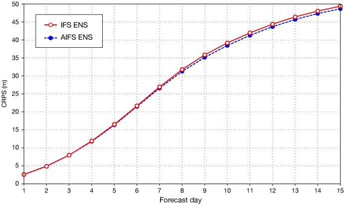
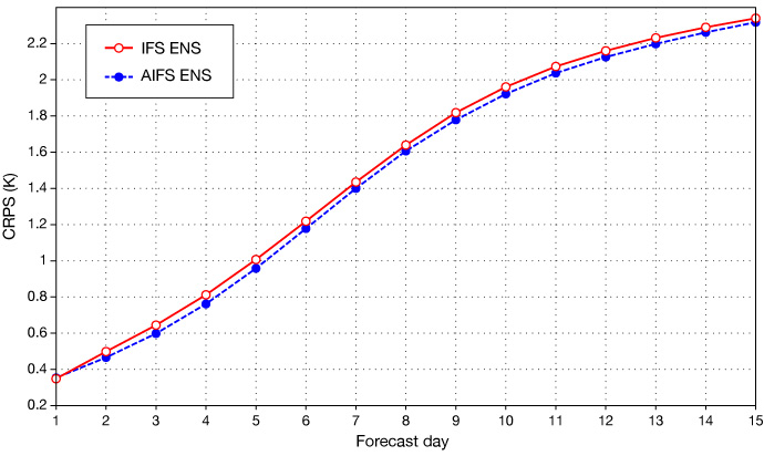
Forecast skill is already comparable with our IFS ENS system. For example, below (Figure 3) we plot the continuous ranked probability score (CRPS) for geopotential height at 500 hPa and temperature at 850 hPa, which quantifies large-scale probabilistic skill.


Figure 3: Continuous ranked probability score (lower is better) for 500 hPa geopotential height (top) and 850 hPa temperature (bottom) showing the IFS ENS (red) and experimental AIFS ENS (blue). Scores are aggregated over the northern hemisphere extratropics and approximately five-month period.
How can you interact with this new model?
Right now, we provide meteograms for any place on Earth, showing the evolution of four variables. Additionally, you can look at plots of ensemble mean and ensemble spread, for a range of variables. These highlight where uncertainty is currently large and small. For both plot types, equivalents exist for the IFS, allowing you to compare and contrast these systems.
The next step, very soon, will be providing all the data, as we now do for the deterministic AIFS, and more plots like the Extreme Forecast Index.
Beyond that, we anticipate further improvements to the model, with our continued emphasis on getting products to users quickly so we can best understand how these new forecasting systems complement the physics-based NWP systems.
Authors
Simon Lang, Matthew Chantry and the rest of the AIFS team (Rilwan Adewoyin, Mihai Alexe, Zied Ben Bouallègue, Mariana Clare, Jesper Dramsch, Christian Lessig, Linus Magnusson, Michael Maier-Gerber, Gert Mertes, Gabriel Moldovan, Ana Prieto Nemesio, Cathal O’Brien, Florian Pinault, Meghan Plumridge, Baudouin Raoult, Mario Santa Cruz, Steffen Tietsche)
Acknowledgements
The AIFS team would like to thank Damien Decremer, Anna Mueller-Quintino, Axel Bonet, Cihan Sahin, Corentin Carton de Wiart, Emma Pidduck, Jenny Wong, Andrea Montani, John Hodkinson, Manuel Fuentes, Martin Suttie, Tiago Quintino and many more at ECMWF for their incredible work in realising this first AIFS ensemble system, and to Mohamed Dahoui for creating the postage stamp heading plot.