
Datasets

Uncoupled ensemble subseasonal reforecasts (ENS-U) with ocean and sea ice boundary conditions derived from observed values at initialisation time. In these experiments, SSTs are specified using daily values from the Operational Sea Surface Temperature and Ice Analysisthat are persisted as anomalies on top of a daily mean SST climatology (1979-2001) derived from the ERA40 reanalysis.
Interval/period: N/A
SNAPSI case study of Northern Hemisphere strong polar vortex case in the stratosphere, initialised on 2022-01-01. TCo319L137 resolution 51-member ensemble, integrated for 70 days.
Examples
Interval/period: N/A
SNAPSI case study of Northern Hemisphere strong polar vortex case in the stratosphere, initialised on 2022-01-01. TCo319L137 resolution 51-member ensemble, integrated for 70 days.
Examples
Interval/period: N/A
Seasonal forecast using CY49R2b with stochastic sea ice scheme active. Used to support the analysis in the paper titled "The impact of stochastic sea ice perturbations on seasonal forecasts" submitted to Weather and Climate Dynamics by K. Strommen, M. Mayer, J. Spaeth and S. Tietsche. Further details in the paper. This forecast can be directly compared against the control counterpart "ikh7".
Examples
Interval/period: N/A
Seasonal forecast using CY49R2b without any stochastic sea ice scheme active. Used to support the analysis in the paper titled "The impact of stochastic sea ice perturbations on seasonal forecasts" submitted to Weather and Climate Dynamics by K. Strommen, M. Mayer, J. Spaeth and S. Tietsche. Further details in the paper. This control forecast can be directly compared to the forecast "imsu", which has stochastic sea ice schemes turned on.
Examples
Interval/period: N/A
The seasonal run (Nov 2018 - Feb 2019) performed on the Oak Ridge Summit supercomputer with a 1.4 km spatial resolution and a 3 hour temporal resolution. Currently only the initial 10 steps have been published as an example, but more data is available on request. Surface fields are available for the entire time range, model level and pressure level fields are available for only the first month. Model levels 1 to 137 are available. Pressure levels 1, 2, 3, 5, 7, 10, 20, 30, 50, 70, 100, 150, 200, 250, 300, 400, 500, 700, 850, 925, 1000 are available.
Interval/period: N/A
This is an global forecast experiment for ALaDyn
Examples
retrieve, class=rd, stream=oper, expver=iglm, type=fc, levtype=sfc, param=2t, date=2000-01-01, time=00:00:00, step=24, target='output.grib'Retrieving 2m-temperature at step 24
retrieve, class=rd, stream=oper, expver=iglm, type=fc, levtype=sfc, param=pr, date=2000-01-01, time=00:00:00, step=1/2/3/4, target='output.grib'Retrieving accumulated total precipitation at steps 1 to 4
Interval/period: N/A
Standalone wave model CY47R1 forced by ERA5 hourly neutral 10m winds, air density, gustiness and sea ice fraction. Native grid is Tco639 (18km), 36 directions, 37 frequencies. No wave data assimilation. Hourly output, including 2d spectra.
Examples
Interval/period: N/A
4-month long 101-ensemble member seasonal attribution experiment (PC98) initialised on 01-November-1997 using the atmosphere-only version of SEAS5 (see Johnson et al., 2019) forced with daily ERA5 SST as in the reference experiment (R98) but with daily SST climatology over the tropical Pacific Ocean.
Examples
Interval/period: N/A
4-month long 101-ensemble member seasonal attribution experiment (PC16) initialised on 01-November-2015 using the atmosphere-only version of SEAS5 (see Johnson et al., 2019) forced with daily ERA5 SST as in the reference experiment (R16) but with daily SST climatology over the tropical Pacific Ocean.
Examples
Interval/period: N/A
4-month long 101-ensemble member seasonal attribution experiment (PC20) initialised on 01-November-2019 using the atmosphere-only version of SEAS5 (see Johnson et al., 2019) forced with daily ERA5 SST as in the reference experiment (R20) but with daily SST climatology over the tropical Pacific Ocean.
Examples
Interval/period: N/A
Polar relaxation experiment run at Tco199 for 46 days over 20 years starting on 12, 16 , 19, 23, 26 , 30 December and 2nd, 6th and 9th January 1999-2018.
Examples
retrieve, class=rd, stream=enfh, expver=iknn, type=pf, number=1/to/4, levtype=sfc, param=2t, date=20191212, hdate=20091212, time=00:00:00, step=24, target='output.grib'Retrieving 2-meter temperature of the hindcast starting on 12 December 2019 for all perturbed members.
Interval/period: N/A
Forecasts using IFS EPS CY47R2 replicating operations (51 members, TCo639, ORCA025Z75). The CO2 concentration was set to 285 ppm. If you are interested in using these data, please let us know by contacting nicholas.leach@physics.ox.ac.uk .
Examples
Interval/period: N/A
Forecasts using IFS EPS CY47R3 replicating operations (51 members, TCo639, ORCA025Z75). The ocean state has had a hydrostatically balanced estimate of anthropogenic influence (warming) since 1850-1900 removed. The CO2 concentration was set to 285 ppm.
Interval/period: N/A
Forecasts using IFS EPS CY47R2 replicating operations (51 members, TCo639, ORCA025Z75). The ocean state has had a hydrostatically balanced estimate of anthropogenic influence (warming) since 1850-1900 removed. The CO2 concentration was set to 285 ppm If you are interested in using these data, please let us know by contacting nicholas.leach@physics.ox.ac.uk .
Examples
Interval/period: N/A
Forecasts using IFS EPS CY47R2 replicating operations (51 members, TCo639, ORCA025Z75). The ocean state has had a hydrostatically balanced estimate of anthropogenic influence (warming) within the CMCC-CM2-HR4 climate model since 1850-1900 removed. The CO2 concentration was set to 285 ppm. If you are interested in using these data, please let us know by contacting nicholas.leach@physics.ox.ac.uk .
Examples
Interval/period: N/A
A 49R1 forecast experiment has been run to generate model fields which can be used to run an offline forward operator for polarimetric radio occultation observations. The fields include convective snow and rain, which are not a standard output for operations. The dates fit to Atmospheric River and Tropical Cyclone cases used for testing the forward operator generating simulated PRO fields (dPhi) and comparing them to observed ones.
Examples
Interval/period: N/A
GraphCast (Google DeepMind): a deep learning-based system developed by Google DeepMind.It is initialised with ECMWF analysis. GraphCast operates at 0.25° resolution.
Interval/period: N/A
GraphCast (Google DeepMind): a deep learning-based system developed by Google DeepMind.It is initialised with ECMWF analysis. GraphCast operates at 0.25° resolution.
Interval/period: N/A
GraphCast (Google DeepMind): a deep learning-based system developed by Google DeepMind.It is initialised with ECMWF analysis. GraphCast operates at 0.25° resolution.
Interval/period: N/A
GraphCast (Google DeepMind): a deep learning-based system developed by Google DeepMind.It is initialised with ECMWF analysis. GraphCast operates at 0.25° resolution.
Interval/period: N/A
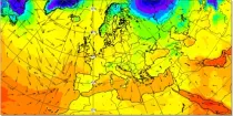
Pangu-Weather: a deep learning-based system developed by Huawei. It is initialised with ECMWF analysis. Pangu-Weather operates at 0.25° resolution.
Interval/period: N/A
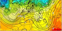
Pangu-Weather: a deep learning-based system developed by Huawei. It is initialised with ECMWF analysis. Pangu-Weather operates at 0.25° resolution.
Interval/period: N/A
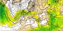
Pangu-Weather: a deep learning-based system developed by Huawei. It is initialised with ECMWF analysis. Pangu-Weather operates at 0.25° resolution.
Interval/period: N/A
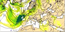
Pangu-Weather: a deep learning-based system developed by Huawei. It is initialised with ECMWF analysis. Pangu-Weather operates at 0.25° resolution.
Interval/period: N/A