Chaos
Chaos theory is one of the major scientific developments of the twentieth century. Chaotic systems are governed by precise deterministic evolution equations, but have unpredictable and seemingly random behaviour. Chaos can occur when these equations are both non-linear and unstable to small perturbations.
Chaos in simple systems
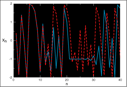
Chaos can be found even in very simple systems; you can even try this one out on your calculator. Choose a number between –2 and 2; call this ‘initial condition’ X1. Calculate the square of X1 and subtract 2; call the result X2. Now do the same thing to X2 (square it and subtract 2) to get X3. Continue to apply the same rule, or algorithm, to generate a long sequence of numbers (we can write this process down as an equation Xn+1 = Xn -2). This system is deterministic – if you start from exactly the same initial condition you will always get exactly the same answer. But because we calculate X-squared it is also non-linear. This is one of the necessary conditions for chaos.
The blue, solid line shows the sequence of numbers X1, X2, X3, etc., up to X40 starting with the initial condition X1 = 0.4. Now suppose we had made a small error in the initial condition and started with X1 = 0.4001. The red, dotted line shows what happens. For the first 10 or so steps all seems well – a small initial error doesn’t affect the result. But then the two sequences of numbers become quite different. This is chaos – small initial differences can lead to completely different predictions.
The formula in this example is a version of an equation, used in the study of population growth, called the logistic equation.
Chaos in the atmosphere
The atmosphere is a chaotic system, and as a result, small errors in our estimate of the current state can grow to have a major impact on the subsequent forecast. Because of the limited number of observations available and the uneven spread of these around the globe, there is always some uncertainty in our estimate of the current state of the atmosphere. In practice this limits detailed weather prediction to about a week or so ahead.
The Lorenz Attractor
One of the fathers of chaos theory is Edward Lorenz. The figure shows the evolution of ensembles of initial points on the famous Lorenz “butterfly” attractor. The two wings of the Lorenz attractor can be imagined as two different weather types, say mild and wet on the left and cold and dry on the right. The initial points represent estimates of the current state of the atmosphere; the arrows show how subsequent forecasts are affected by the small initial errors. The three panels show how the effect of these errors can vary depending on the initial “true state”. When we are in a predictable state (top left panel), small errors in the starting conditions will not affect the forecast: we can be confident that the weather will become cold and dry. If, however, we are in a less predictable situation (top right panel), the points stay together only for a limited time before diverging. While we can be confident of the forecast for a few days ahead, we cannot be sure if it will ultimately stay wet or become drier. Sometimes the situation is so unpredictable that we can have little confidence in the outcome even a short period ahead (bottom left panel).

Ensemble prediction
Accepting the findings from chaos theory about the sensitivity of the prediction to uncertainties in the initial conditions, it is becoming common now to run in parallel a set, or ensemble, of predictions from different but similar initial conditions. The ECMWF Ensemble Prediction System (EPS) provides a practical tool for estimating how these small differences could affect the forecast. The ECMWF weather prediction model is run 51 times from slightly different initial conditions. To take into account the effect of uncertainties in the model formulation, each forecast is made using slightly different model equations.
The 51 scenarios can be combined into an average forecast (the ensemble-mean) or into a small number of alternative forecasts (the clusters), or they can be used to compute probabilities of possible future weather events.
Risk management
The EPS can be used as a quantitative tool for risk assessment in a range of weather-sensitive commercial and humanitarian activities. The potential economic value of the EPS can be much higher than that of a forecasting system based on only a single deterministic forecast.
Different users will be more or less sensitive to adverse weather and so will benefit differently from weather forecasts. The figure shows an example of the potential economic value of forecasts to a range of users (represented along the horizontal axis). Value (which ranges between 0 for a forecast with no information to 1 for perfect forecasts) is higher for probabilistic predictions based on the EPS (red line) than for deterministic predictions based on the control forecast (blue line) or on the ensemble-mean forecast (green line). These results are for 5-day forecasts of heavy precipitation (more than 10 mm/day) over Europe for winter 1999-2000. Value is calculated using a simple cost-loss decision model.
More information can be found in the following ECMWF Newsletter articles:
- Richardson, D. S. 1998: Obtaining economic value from the EPS ECMWF Newsletter 80, Summer 1998.
- Buizza, R. 2001: Weather risk management with the ECMWF ensemble prediction system. ECMWF Newsletter 92, Autumn 2001