Datasets

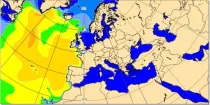
Significant wave height can be shown to correspond to the average wave height of the top one-third highest waves. The wave period of windsea is generally <10s,...

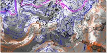
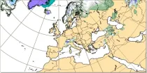
850 hPa wet-bulb potential temperature is commonly used to identify air masses and a strong gradient of wet bulb potential temperature is indicative of fronts between two different air masses...

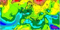
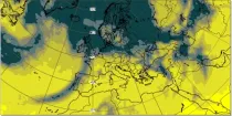
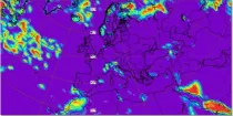
The simulated water vapour images generally focus on the upper troposphere. These charts can often indicate dynamical forcing mechanisms (responsible for cyclogenesis) or convective development (related to potential instability)...

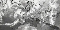
These products display cloud-related fields from the model in a format that is very familiar to forecasters and that they are used to interpreting. They can easily be compared to actual satellite imagery...

The simulated water vapour images generally focus on the upper troposphere. These charts can often indicate dynamical forcing mechanisms (responsible for cyclogenesis) or convective development (related to potential instability)...

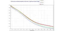
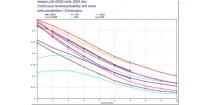
These diagrams compare Continuous Ranked Probability Skill Scores (CRPSS) of ECMWF with ...

These diagrams compare the Brier Skill Scores (BSS) and the  Continuous Ranked Probability ...

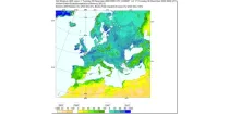
Snow depth is computed using two model parameters - these represent the liquid water equivalent of snow lying on the ground, and the average density of that snow layer...

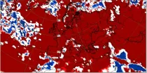
Soil moisture handling in the model is complex, and could be highlighted in many ways. Here a 'relativistic' approach is used for display, showing not absolute values, but instead...

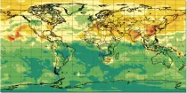
Specific humidity gives an indication of the amount of moisture within a sample of air (in g of water vapour within a kg of air, g kg⁻¹). The chart shows the specific humidity at 1000 hPa and 925 hPa levels and...

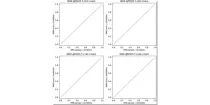
These reliability diagrams show the ensemble spread of different global models for temperature ...

Stratosphere relaxation experiment run at Tco199 for 46 days over 20 years starting on 12, 16 , 19, 23, 26 , 30 December and 2nd, 6th and 9th January 1999-2018.

Examples

Retrieving 2-meter temperature of the hindcast starting on 12 December 2019 for all perturbed members.

The climatological bias-correction experiment consists of sub-seasonal hindcasts performed with IFS cycle 48r1, in which a fixed tendency correction is applied to account for systematic model error. Hindcasts are initialised on the 15th of each month from 1989 to 2016 and integrated forward for 32 days. For each start date, an ensemble of 10 members is generated, comprising one unperturbed control and nine perturbed members to sample initial-condition uncertainty. The model is run at TCo319 horizontal resolution with 137 vertical levels.

The control experiment consists of sub-seasonal hindcasts performed with IFS cycle 48r1, without any explicit bias correction or model-error tendencies applied. Hindcasts are initialised on the 15th of each month from 1989 to 2016 and integrated forward for 32 days. For each start date, an ensemble of 10 members is generated, comprising one unperturbed control and nine perturbed members to sample initial-condition uncertainty. The model is run at TCo319 horizontal resolution with 137 vertical levels.

The flow-dependent bias-correction experiment consists of sub-seasonal hindcasts performed with IFS cycle 48r1, in which model-error tendencies are estimated online using neural networks. Hindcasts are initialised on the 15th of each month from 1989 to 2016 and integrated forward for 32 days. For each start date, an ensemble of 10 members is generated, comprising one unperturbed control and nine perturbed members to sample initial-condition uncertainty. The model is run at TCo319 horizontal resolution with 137 vertical levels.

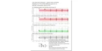
This chart shows the 7-day mean anomalies of four forecast parameters for the Sub-seasonal range ...

CAMS sulphur dioxide forecasts

Sunshine for any point is assessed using the model representation of cloud layers to decide how much direct solar (shortwave) radiation reaches the Earth's surface...

This chart shows probabilities for the 7-day mean anomalies of surface temperature to be in ...

This chart shows probabilities that 7-day mean surface temperatures (from the 101 forecast ...

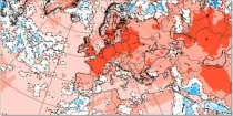
This chart shows 7-day mean anomalies of surface temperature from the ECMWF Sub-seasonal range ...

The step=0 data from these experiments provides Tco1279 initial conditions derived from ERA5 and IFS CY48R1.1. The type=pf members include perturbations from the ERA5 EDA and singular vectors calculated using IFS CY48R1.1.

Examples

Coupled ensemble reforecasts using the ECMWF IFS cycle 47r3, configured as follows. The atmosphere is set up with 15 ensemble members, 137 model levels and run on Tco199 cubic octahedral reduced Gaussian grids. The IFS is coupled hourly to a 75-level NEMO v3.4 ocean model and an LIM2 sea ice model, both utilising the ORCA025 tripolar grid with a grid spacing of approximately 0.25 degrees. The ocean and atmosphere are fully coupled throughout the 46-day forecast, producing output every 12 hours. Fifteen reforecasts are used.

Coupled ensemble reforecasts using the ECMWF IFS cycle 47r3, configured as follows. The atmosphere is set up with 15 ensemble members, 137 model levels and run on Tco199 cubic octahedral reduced Gaussian grids. The IFS is coupled hourly to a 75-level NEMO v3.4 ocean model and an LIM2 sea ice model, both utilising the ORCA025 tripolar grid with a grid spacing of approximately 0.25 degrees. The ocean and atmosphere are fully coupled throughout the 46-day forecast, producing output every 12 hours. Fifteen reforecasts are used.

Coupled ensemble reforecasts using the ECMWF IFS cycle 47r3, configured as follows. The atmosphere is set up with 15 ensemble members, 137 model levels and run on Tco319 cubic octahedral reduced Gaussian grids. The IFS is coupled hourly to a 75-level NEMO v3.4 ocean model and an LIM2 sea ice model, both utilising the ORCA025 tripolar grid with a grid spacing of approximately 0.25 degrees. The ocean and atmosphere are fully coupled throughout the 46-day forecast, producing output every 12 hours. Fifteen reforecasts are used.