On 14 October 2020, the European Flood Awareness System (EFAS) launched a new cycle upgrade, EFAS version 4.0. This was a step-change in EFAS. For the first time, the LISFLOOD hydrological model, the ‘engine’ of EFAS, was calibrated using sub-daily steps and it is now used with sub-daily steps in all hydrological simulations throughout the system.
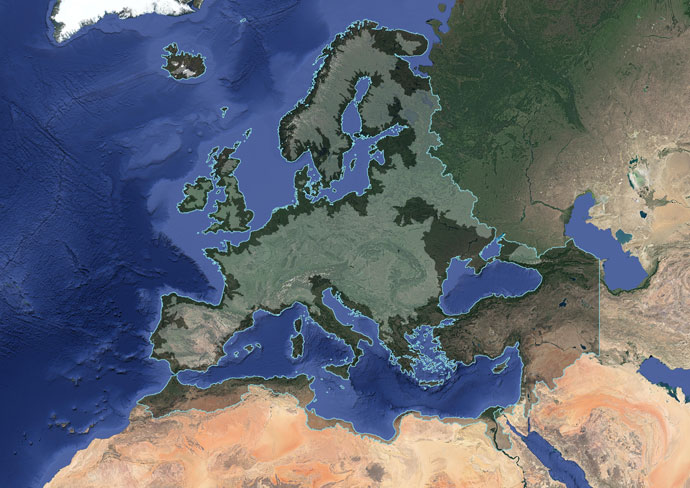
The EFAS domain includes 66 countries. For EFAS version 4.0, a total drainage area of 4M km2 was calibrated so that the hydrological representation of those catchments can be as accurate as possible (Figure 1). This resulted in a marked improvement in the hydrological simulations for most catchments, except in strongly regulated catchments, where the new calibration did not bring much change.
This article introduces the new 6‑hourly calibration of the LISFLOOD hydrological model and provides a summary of its performance.
%3Cstrong%3EFIGURE%201%3C/strong%3E%20Map%20of%20the%20EFAS%20domain%20(dark%20shade)%20and%20calibration%20extent%20(light%20shade).FIGURE 1 Map of the EFAS domain (dark shade) and calibration extent (light shade).
What is EFAS?
EFAS is an operational pan-European flood forecasting system funded by the European Commission through its Copernicus programme. The aim of EFAS is to support preparatory measures before major flood events strike, particularly in large transnational river basins and throughout Europe in general.
EFAS is a component of the Copernicus Emergency Management Service (CEMS). Since the beginning of its operational implementation in 2012, it has been providing flood forecast information to 116 national hydro-meteorological services across Europe, the European Commission’s Emergency Response and Coordination Centre (ERCC), and other research institutes. EFAS is managed by the EU Joint Research Centre (JRC) and is delivered by four centres run by different consortia:
Computational centre (EFAS-COMP) It is responsible for producing forecasts and hosting the EFAS-Information System platform. It is operated by ECMWF.
Dissemination centre (EFAS-DISS) It provides a daily analysis of EFAS forecasts and disseminates the information to EFAS partners and the ERCC. It is coordinated by the Swedish Meteorological and Hydrological Institute and also comprises the Dutch Rijkswaterstaat and the Slovak HydroMeteorological Institute.
Hydrological data collection centre (EFASHYDRO) It collects historical and real-time river discharge and water level data across Europe and makes them available to EFAS-COMP. It is delivered by the Environmental and Water Agency of Andalucía (REDIAM) and Soologic Technological Solutions SL.
Meteorological data collection centre (EFASMETEO) It collects historical and real-time meteorological data across Europe and provides them in real-time to drive the EFAS modelling chain. It is composed of KISTERS AG and the German national meteorological service (Deutscher Wetterdienst, DWD).
As part of the EFAS computational centre’s role, ECMWF is also responsible for developing and integrating into operation any improvement in the forecast model chain, and for developing, managing and running the EFAS web and data services.
Medium-range forecasts in EFAS
EFAS medium-range ensemble flood forecasts are generated by cascading an ensemble of meteorological forecasts (from ECMWF, DWD and COSMO-LEPS from the COSMO consortium), meteorological and hydrological observations, land surface information and model parameters (static maps) through a deterministic hydrological model (LISFLOOD).
The resulting ensemble flood forecasts are postprocessed to produce all EFAS products. The products, including flood highlights of different severity levels, are made available to EFAS-DISS and EFAS users as maps and graphs. Three severity levels are highlighted, corresponding to forecasts of floods expected to exceed flood peaks with return periods of 2, 5, and 20 years (a return period indicates the average number of years expected between two floods of the predicted magnitude). Finally, EFAS-DISS duty forecasters analyse the flood summary maps and issue notifications to registered users of the concerned region to inform them of possible upcoming events (Figure 2).
%3Cstrong%3EFIGURE%202%3C/strong%3E%20EFAS%20flood%20forecast%20and%20notification%20process.FIGURE 2 EFAS flood forecast and notification process.
A new 6-hourly calibration
Like other operational forecasting systems, EFAS is always evolving, but the October 2020 upgrade included a step-change in EFAS hydrological modelling for medium-range forecasts. For the first time, the LISFLOOD hydrological model was calibrated at 6‑hourly steps over the EFAS pan-European domain, compared to 24‑hourly steps previously. At the same time, all hydrological medium-range simulations are produced at sub-daily steps, so that the timing of the start and peak of flood events can be better anticipated.
Upgrade of the hydrological model
LISFLOOD has been developed at the JRC since 2000 and has been used for operational flood forecasting at the pan-European scale since the early days of EFAS. Since 2019 the model is fully open source and the code is developed and maintained through a GitHub repository by the JRC (https://ec-jrc.github.io/lisflood/), with support from the EFAS-COMP team at ECMWF.
LISFLOOD is a fully distributed hydrological model, which explicitly considers the spatial distribution of physical properties across catchments and provides estimates of river discharge on the entire geographical domain. Driven by meteorological forcing data (precipitation, temperature, potential evapotranspiration, and evaporation rates for open water and bare soil surfaces), LISFLOOD calculates a complete water balance for every grid cell within the EFAS domain, currently on a 5x5 km grid. Processes simulated include snowmelt, soil freezing, surface runoff, infiltration into the soil, preferential flow, redistribution of soil moisture within the soil profile, drainage of water to the groundwater system, groundwater storage, and groundwater base flow. Runoff produced for every grid cell is then routed through the river network using a kinematic wave approach. The model also includes options to simulate lakes and reservoirs.
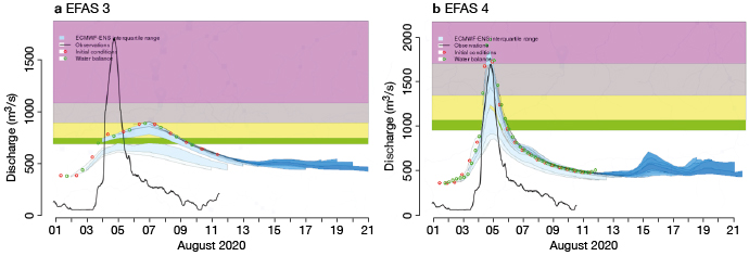
For EFAS 4, LISFLOOD was upgraded to run sub-daily time steps (6-hourly), routing of flood waves in rivers was improved and the handling of model state files was refined. The upgrades allowed for better representation of hydrology in small to medium size catchments (Figure 3) and for the use of more realistic parameters in the calibration process.
%3Cstrong%3EFIGURE%203%3C/strong%3E%20Example%20of%20the%20improvement%20to%20simulated%20hydrographs%20between%20(a)%20EFAS%203%20and%20(b)%20EFAS%204%20for%20the%20river%20Inn%20at%20M%C3%BChldorf%20(Germany).%20The%20observed%20discharge%20is%20represented%20by%20the%20black%20line,%20LISFLOOD%20outputs%20are%20represented%20by%20the%20green%20and%20red%20dots.FIGURE 3 Example of the improvement to simulated hydrographs between (a) EFAS 3 and (b) EFAS 4 for the river Inn at Mühldorf (Germany). The observed discharge is represented by the black line, LISFLOOD outputs are represented by the green and red dots.
New 6-hourly forcing fields
By upgrading the full EFAS medium-range modelling chain to a 6‑hourly timestep, all forcing fields, including observed meteorological data to simulate initial conditions, needed to also be produced at the finer time step. For the LISFLOOD model, this includes gridded maps of precipitation, average air temperature, evaporation rate from free water surface and bare soil surface, and potential evapotranspiration for reference crop surfaces.
In EFAS, the meteorological data collection centre (EFAS-METEO) collects datasets of historical and real-time in-situ meteorological observations on a 24/7 basis from 22 data providers over more than 40k stations and 70k sensors, and it interpolates them to the 5 km hydrological model grid.
For the calibration of EFAS 4, EFAS-METEO produced new datasets with 6-hourly gridded meteorological maps of precipitation and average surface air temperature using point observations for the period 1990–2017 on the model’s 5 km spatial resolution. Because of the sparsity of meteorological data such as wind speed, solar radiation or humidity at a 6‑hourly time step, estimates of potential evapotranspiration were made using the Penman-Monteith equation with daily data, and then disaggregated using the same evaporation rates for each time step to produce 6-hourly grids.
New daily and sub-daily discharge dataset
The EFAS hydrological data collection centre (EFASHYDRO) collects historic and real-time river discharge and water level data across Europe from 44 data partners. Metadata such as name, location and upstream drained area are also collected and maintained. Data from more than 1,800 active stations are collected on a 24/7 basis either as water levels and/or discharge at different temporal resolution, then quality checked and resampled at 1-, 6- and 24‑hour time steps. Water level data are transformed to discharge data (the information which is required by LISFLOOD) when rating curves are provided by EFAS partners.
For the calibration of EFAS 4, a dataset containing daily and 6‑hourly discharge data at river gauges for the period 1990–2017 was put together at ECMWF, based on data provided by EFAS-HYDRO.
Ancillary maps
LISFLOOD requires a wide range of spatially distributed input parameters and variables such as topography, soil type, land use, channel geometry, and river network. The pan-European setup of LISFLOOD uses a 5 km grid on a Lambert Azimuthal Equal Area projection. EFAS configuration maps were created by the Joint Research Centre (JRC) of the European Commission from various European databases with emphasis on having a homogeneous base all over Europe.
For EFAS 4, the LISFLOOD domain area was slightly extended to include the Jordan catchment. The river network in the Balkans was also improved to better represent physical rivers in the region, with updates to the channels’ geometry reflecting the changes done to the drainage network. The LISFLOOD model for EFAS 4 includes 1,423 reservoirs and 210 lakes. Compared to the previous EFAS 3 version, three additional reservoirs were added on the Sava river downstream of Zagreb to better represent the effects of large retention areas.
Calibration stations
LISFLOOD calibration stations were selected from the list of 2,927 river gauging stations with discharge data that was available in the EFAS-HYDRO database in July 2018, when calibration work began. Stations were located on the LISFLOOD 5 km drainage network using a semi-automatic procedure and additional manual checks. Available discharge data were then quality checked to exclude stations where discharge data showed issues with instrumentation, rating curves or water release from reservoirs.
Stations where a minimum of four years of good-quality discharge data were available were selected as calibration points. For the sake of representativeness and to reduce the computation time of the calibration, stations located close to others along the same river (i.e. stations with a difference in drained area smaller than 200 km2) and with the same data quality were excluded in favour of the station with the longest data period or the largest drainage area.
The selection procedure produced a list of 1,137 calibration stations in 215 different catchments, 406 with 6‑hourly and 731 with daily observed discharge time series. In total, 44.5% of the EFAS domain area belongs to a calibrated catchment, corresponding to 4 million km2 over 9 million km2, with the catchment area of the stations varying from 468 km2 (Ishem catchment, Albania) to 807,000 km2 (Danube catchment, Romania) and a median area of 3,000 km2.
Compared to the EFAS 3 system, the number of calibration points increased by 426 stations, up from 711 in the previous calibration exercise. However, some of the already existing calibration stations are now providing 6‑hourly data and thus different data were used in the EFAS 4 calibration, often on significantly shorter periods.
Calibration methodology
Like most rainfall-runoff models, the equations of the LISFLOOD hydrological model include a range of parameters. Some of these can be determined from physical data, such as reservoir storage-elevation curves, or the drainage area of watersheds. Others vary from one area to another based on changes in climatology and physical factors, e.g. hydraulic soil properties. Some model parameters require calibration, which is generally obtained by tuning parameter values based on a comparison between simulated and observed discharge (Q) at river gauges. This tuning process generally aims to minimise errors in the volume and timing of simulated flow over a multi-year period.
A set of 14 model parameters was selected for calibration following recommendations from previous work on the LISFLOOD model and its application to EFAS. The parameters control snow accumulation and snow melting, overland flow, percolation to the lower groundwater zone, the residence time of the upper and lower groundwater zone, lakes, reservoirs and channel routing. Parameter spaces were defined by physically reasonable lower and upper limits for physically based parameters and largest admissible ranges for empirical parameters.
For EFAS 4 calibration, an Evolutionary Algorithm (EA) was used to generate sets of model parameters and the modified Kling-Gupta efficiency (KGE’) was selected as the objective function (or goodness-of-fit measure) as it provides a way to achieve balanced improvement of simulated mean flow, flow variability, and correlation.
A number of calibration stations were available along the same rivers. This offered information on nested catchments, which is very important for a distributed hydrological model calibration. However, it came with an additional challenge in terms of calibration strategy and run time, as data was generally a mix of 6‑hourly and daily discharge observed over different time periods. This was solved by dividing the EFAS domain in 1,137 sub-catchments or inter-catchments and by performing the calibration through a catchment-based parallelisation of the model domain.
Each sub-catchment was calibrated separately but using a multisite cascading calibration (MSCC) approach, where the calibrated discharge from upstream river basins was used as input for downstream ones. The calibration was iteratively performed from upstream to downstream, from the catchment with the smallest area to the largest one, as flow routing calculations must be carried out in a serial manner along the mainstream of a river basin.
To run the parameter optimisation procedure, the LISFLOOD model was run at 6-hourly steps everywhere. However, the objective function (or goodness-of-fit measure) was calculated over a daily-aggregated time series for calibration points with daily observations, to allow a fair comparison between simulated and observed discharge data. This dual calibration strategy (both at 6‑hourly and daily time steps) was critical to guarantee the best possible geographical coverage as 6‑hourly river discharge data was not available everywhere.
Hydrological model performance
The calibration process resulted in 14 new parameter maps over the pan-European EFAS extent, one per calibrated parameter. For each sub-catchment domain, the parameters identified by the calibration procedure were used in all grid cells, while for areas not covered by the calibration stations, default parameters were used instead. Most of the parameters in LISFLOOD act as multipliers for the ancillary maps describing the geo-physical properties of the catchments, so even if a single value is used for all model pixels in a catchment, spatial variability of the model parameters is preserved through the ancillary maps. Parameter maps were then used to execute a continuous simulation forced with observations for the period Jan 1990 – Dec 2017. The simulated discharge was then compared against observed discharge from the 1,137 calibration stations, excluding the year 1990 so that the impact of the initial conditions did not affect the comparison. For calibration stations with daily data, 6‑hourly LISFLOOD time series were aggregated at daily steps before the comparison with the observations.
One important aspect of a hydrological model performance evaluation is to use data which have not been used during the calibration exercise, so that the evaluation is a fair analysis of the model behaviour. This is often achieved using a ‘split sample approach’, where the hydrometeorological observational record is split into two independent periods, one used to optimise the parameters through calibration, and one used to evaluate the model behaviour. This could not be fully adopted for EFAS 4 for two main reasons. First, although each calibration station was calibrated separately, observational periods were generally different, making it impossible to define the same non-overlapping periods for all calibration points along the same river. Second, some calibration stations had only four years of available data, which is the shortest necessary duration to achieve a robust parameter optimisation, and no data were left for evaluation. This meant that no observational record was available to conduct an independent evaluation for those stations. As a compromise, the calibration was done using a sub-set of the observation record in most of the stations, but the hydrological model performance was evaluated on the full available discharge record (including the data used for the calibration).
Hydrological model performance was measured using the modified Kling-Gupta efficiency (KGE’), the same metric as that used for model calibration. The KGE’ is an expression of the distance from the point of ideal model performance in the space described by three components: correlation, variability bias and mean bias. It can vary between any negative number and 1, where 1 indicates perfect agreement between simulations and observations.
All three components of KGE’ represent desirable characteristics of the hydrological regime in the context of EFAS: correlation evaluates the flow timing, of paramount importance for EFAS to issue timely warnings. Variability bias measures the statistical variability, ensuring that peaks are correctly reproduced by the system. And mean bias describes the long-term water balance, important for any hydrological application. It is important to remember that although the length of the model run is the same for all stations, discharge data availability is uneven, and therefore KGE’ is computed using different data periods for each station across the EFAS domain.
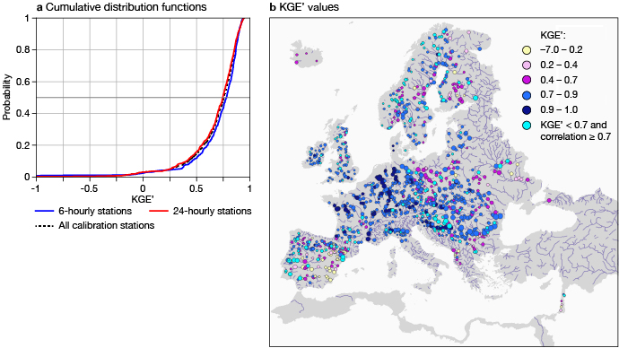
%3Cstrong%3EFIGURE%204%3C/strong%3E%20Hydrological%20model%20performance%20of%20EFAS%20v4.0%20as%20described%20by%20the%20modified%20Kling-Gupta%20efficiency%20score%20(KGE%E2%80%99)%20calculated%20over%201991%E2%80%932017,%20showing%20(a)%20the%20cumulative%20distribution%20function%20(CDF)%20for%20all%20calibration%20stations,%206-hourly%20calibration%20stations%20and%2024-hourly%20calibration%20stations%20and%20(b)%20the%20KGE%E2%80%99%20skill%20score%20for%20each%20calibration%20station%20as%20coloured-coded%20symbols.%20Stations%20with%20KGE%E2%80%99%20%3C%200.7%20and%20correlation%20%E2%89%A5%200.7%20are%20shown%20separately.%20The%20size%20of%20the%20dots%20is%20proportional%20to%20the%20drained%20area%20of%20the%20calibration%20station.FIGURE 4 Hydrological model performance of EFAS v4.0 as described by the modified Kling-Gupta efficiency score (KGE’) calculated over 1991–2017, showing (a) the cumulative distribution function (CDF) for all calibration stations, 6-hourly calibration stations and 24-hourly calibration stations and (b) the KGE’ skill score for each calibration station as coloured-coded symbols. Stations with KGE’ 0.7 and correlation ≥ 0.7 are shown separately. The size of the dots is proportional to the drained area of the calibration station.
The hydrological model performance over 1991–2017 as expressed by the KGE’ is shown in Figure 4. Overall, around 50% of the calibration stations achieve a KGE’ greater than 0.75, a high value for model performance compared to an optimum of 1. There is very little difference regarding the performance of stations calibrated at a 6-hourly or daily time step, although the former tend to have a slightly better score (Figure 4a). Generally, performance is relatively uniform across the EFAS pan-European domain (Figure 4b). However, areas of higher skill are found in large parts of Central Europe and the main European rivers, whilst lower skill is mostly concentrated in catchments with strongly regulated rivers, like in the Iberian Peninsula. Stations with KGE’ < 0.7 and correlation ≥ 0.7 are also highlighted to show stations that might have lower KGE’ due to systematic bias, but still have high correlation. Correlation is particularly important for EFAS given that forecasts are compared to model thresholds, so they are bias invariant to a large extent.
Comparing hydrological model performance
For the fairest comparison possible between EFAS versions 3 and 4, the hydrological model performance score KGE’ was calculated on simulations using the same meteorological forcing data (but aggregated to daily forcing for EFAS 3) over 1990–2017. For EFAS 4, scores were calculated on river discharge averaged over 24 hours to be comparable to the 24‑hourly simulation of EFAS 3 (also matching the calibration time step of EFAS 3). Note that calculating KGE’s over daily discharge slightly increases the score of EFAS 4.
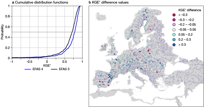
Overall, EFAS 4 shows a marked improvement in the hydrological performance compared with EFAS 3, with more stations achieving a higher KGE’ score as shown by the cumulative distribution function. About 60% of stations have a KGE’ of 0.75 or higher, against only 40% for EFAS 3 (Figure 5a). Improvements are found over most of the EFAS domain, with the exception of some stations in Scandinavia, Spain and central Europe (Figure 5b). Causes for skill score degradation are varied. In the Elbe catchments, EFAS 4 calibration could only be conducted with a much shorter period of data (down to only four years on the main Elbe river, using 6‑hourly records) during a period without major flood events, compared with a much longer and hydrologically diverse calibration for EFAS 3. Catchments in Scandinavia and Spain have a large number of reservoirs, which can be challenging to model at 6-hourly steps. Finally, the LISFLOOD routing scheme, which does not flatten peaks during flood propagation, is slightly penalised by the 6‑hourly time step over large river basins in flat areas. This is because higher and more accurate peak floods from small and medium size upstream catchments are now produced by the model but are not properly propagated downstream. This is the case, for example, in the Danube.
%3Cstrong%3EFIGURE%205%3C/strong%3E%20Change%20in%20the%20EFAS%20hydrological%20model%20performance%20between%20v3%20and%20v4%20as%20described%20by%20the%20modified%20Kling-Gupta%20efficiency%20score%20(KGE%E2%80%99)%20calculated%20on%20daily%20river%20discharge%20over%201991%E2%80%932017,%20showing%20(a)%20the%20cumulative%20distribution%20function%20(CDF)%20for%20EFAS%203%20and%20EFAS%204%20and%20(b)%20for%20each%20common%20calibration%20station,%20the%20difference%20in%20KGE%E2%80%99%20values%20for%20EFAS%204%20and%20EFAS%203%20as%20colour-coded%20symbols.%20Blue%20(red)%20shades%20highlight%20stations%20where%20EFAS%204%20performs%20better%20(worse)%20than%20EFAS%203.%20The%20size%20of%20the%20dots%20is%20proportional%20to%20the%20drained%20area%20of%20the%20calibration%20station.FIGURE 5 Change in the EFAS hydrological model performance between v3 and v4 as described by the modified Kling-Gupta efficiency score (KGE’) calculated on daily river discharge over 1991–2017, showing (a) the cumulative distribution function (CDF) for EFAS 3 and EFAS 4 and (b) for each common calibration station, the difference in KGE’ values for EFAS 4 and EFAS 3 as colour-coded symbols. Blue (red) shades highlight stations where EFAS 4 performs better (worse) than EFAS 3. The size of the dots is proportional to the drained area of the calibration station.
What next for EFAS
The release of EFAS version 4 marks a milestone in EFAS development, delivering a first system calibrated with sub-daily data. The hydrological skill improvement provided by the new calibration and the higher time resolution of the products based on LISFLOOD outputs will allow for a timelier notification of the beginning and peak of predicted flood events, and for EFAS users to better understand and explore flood forecasts.
As with any operational forecasting system, EFAS development never stops. Even though the new EFAS version 4 has only just been released, the EFAS-COMP team at ECMWF has already started working on the next exciting new development: an almost 10‑fold increase in the number of model cells, with the spatial resolution going from a 5 km grid to a ~1.8 km (1 arcminute) grid.
Further reading
Arnal, L., S.-S. Asp, C. Baugh, A. de Roo, J. Disperati, F. Dottori et al., 2019: EFAS upgrade for the extended model domain – technical documentation. EUR 29323 EN, Publications Office of the European Union, Luxembourg, ISBN 978-92-79-92881-9, doi:10.2760/806324, JRC111610.
Gupta, H., H. Kling, K. Yilmaz & G. Martinez, 2009: Decomposition of the Mean Squared Error and NSE Performance Criteria: Implications for Improving Hydrological Modelling. Journal of Hydrology, 377, 80–91, doi:10.1016/j. jhydrol.2009.08.003.
Kling, H., M. Fuchs & M. Paulin, 2012. Runoff conditions in the upper Danube basin under an ensemble of climate change scenarios. Journal of Hydrology, 424–425, 264–277, doi:10.1016/j.jhydrol.2012.01.011.
Mazzetti, C. & C. Prudhomme, 2018: Major upgrade for European flood forecasts. ECMWF Newsletter No. 157, 3.