The following article was posted on 6 June 2014, to mark the 70th anniversary of the D-Day landings
Revisiting the meteorology of the D-Day period, using a modern analysis and forecasting system
Introduction
Weather forecasts critical to the success of the D-Day landings of 6 June 1944 were made on the nights of 3/4 and 4/5 June 1944:
- forecasts for conditions on 5 June made on the evening of 3 June and confirmed early in the morning of 4 June;
- forecasts for conditions on 6 June made on the evening of 4 June and confirmed early in the morning of 5 June.
The first of these two forecasts, presented to the Supreme Commander of the Allied Forces in Europe, General Eisenhower, by his meteorological advisor, Group Captain J.M. Stagg, led to the postponement of the invasion planned for 5 June; the second enabled Eisenhower to make the decision to go ahead the following day.
From source material (Figure 1) such as the book written later by Stagg himself and the multiple accounts presented at a 40th anniversary symposium held by the California Chapter of the American Meteorological Society (AMS), a picture emerges of how three separate teams, from the Met Office, the Admiralty and the US Army Air Forces, first made separate forecasts and then sought consensus - an early example of what today we refer to as ensemble forecasting. On 3 June the teams initially split two-to-one in favour of conditions leading to postponement; the following day it was initially a two-to-one split in favour of conditions that would allow the invasion to proceed. Demanding military requirements, stormy weather in the North Atlantic and associated fronts moving up the English Channel combined to make forecasting far from easy, and decisions were finely balanced.

Figure 1 Principal sources of background information and original charts used in this article.
Although conditions were some way from meeting the original military requirements, the fundamental objective of the D-Day operation was achieved. Had the decision not been made to go ahead with the landings on 6 June or thereabouts, the next occasion when tides (but not moon) were favourable was almost two weeks later. On 17th June there was consensus among the forecast teams that weather conditions would be calm, a forecast that most likely would have had calamitous consequences had it been used to decide on a delayed invasion.
Reconstructing the weather conditions for the critical days
Today, the science and technology of weather forecasting is far removed from that of seventy years ago. Forecasting beyond a few hours ahead nowadays relies on automated procedures for processing digitised observations to give a snapshot of the state of the atmosphere. This is used to initiate a computerised model of the atmosphere that projects the information forward in time to form the forecast. The initial snapshot, known as the “analysis”, itself depends on the atmospheric model; it is constructed by blending the latest observations with a “background” forecast initiated from an analysis made some time earlier. As time goes by, this process of “data assimilation” produces a picture of how the weather has evolved, built up by the succession of analyses.
The European Centre for Medium-Range Weather Forecasts (ECMWF), and organisations in Japan and the USA, have been active in programmes of global “reanalysis” in which the observations taken over past decades are reprocessed using modern data assimilation systems to produce complete historical records of the atmosphere, for use in a wide range of meteorological and climatological studies.
Ten years ago, ECMWF had completed ERA-40 a reanalysis that provided a three-hourly record of conditions back to 1957, when the atmospheric observing system was enhanced in preparation for the International Geophysical Year. To mark the retirement of our then Director, David Burridge, who was born in June 1944, and recognising the challenge and interest in reanalysing the meteorological conditions of the D-Day period as its sixtieth anniversary approached, we stepped back a further few years, and applied a slightly updated version of the ERA-40 data assimilation system to reconstruct the weather of June 1944. This was not a comprehensive study; instead we simply made use of existing tools and a quite limited number of readily available observations. Although far from perfect, the results agreed in the broadest terms with the historical record.
Ten years on, a new opportunity to re-examine the meteorology and sea-state conditions for June 1944 presents itself. ECMWF has recently completed ERA-20C, a reanalysis for the period from 1900 to 2010 assimilating surface pressure and marine surface wind observations. This follows the first reanalysis of this type, the NOAA-CIRES 20th Century Reanalysis. We are also currently producing a second reanalysis that builds on ERA-20C from 1939 onwards by including upper-air observations. This second reanalysis provides the basis for the results presented here.
The ERA-CLIM reanalysis system
The reanalyses we study were instigated as part of a multi-partner project, ERA-CLIM, whose activities continue under the current ERA-CLIM2 project, both funded by the European Union under its Seventh Framework Programme. The ERA-CLIM system for assimilating observational data uses the version of the ECMWF operational system run operationally from June 2012 to June 2013, but with a number of modifications needed to make production of such a long data record affordable, or to account for a coverage of observational data that is initially sparse and changes significantly over time.
The assimilation system thus uses a background model with a horizontal resolution of about 125 km, as used for ERA-40, rather than the much finer 16 km resolution currently employed by ECMWF for operational forecasting. It is novel in using a cycling period as long as 24 h, determining for each day an adjustment of the background forecast for 09 UTC that makes a new forecast from that time fit optimally the observations made over the following 24 h. This is illustrated schematically in Figure 2. An ensemble of ten assimilations for the period was first run using perturbed surface observations and sea-surface temperatures. This provided an estimate of uncertainty that enabled the observational data to be given the appropriate weight in the assimilation procedure. Single reanalyses were then run using optimised settings, both with and without the upper-air data.
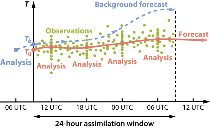
Figure 2 Schematic form of the ERA-CLIM data assimilation.
Forecasts were run routinely to ten days ahead from 00 UTC each day as part of the production system, as their accuracy provides another indicator of analysis quality. Specific to our study of June 1944, forecasts were also run to three days ahead from 00 UTC and 12 UTC using the operational 16 km resolution to enhance the realism of wind and cloud fields. This was done both for 2 to 7 June to cover the critical D-Day period and for 18 to 23 June to cover the long-lasting, destructive and originally unpredicted storm that occurred at the time the landings might have been attempted had they not been made on 6 June. These down-scaled winds were used to drive a separate ocean-wave model with spatial resolution of about 11 km, to provide reconstructions of the sea-state over these two key periods.
An important point to keep in mind is that these forecasts benefit from the availability of observations 21 h into the future in the case of 12 UTC starting times and 9 h into the future for the 00 UTC starting times. They thus do not directly represent what a real-time operational forecasting system could have produced in June 1944 had modern forecasting methods (but not modern observations) been available. Although allowance can be made for this by inflating the lead times of the forecast, we still do not know exactly which observations were available to the forecasting teams that reported to Stagg, nor do we have access to all of the data.
The observations
The observations assimilated in these reanalyses come from five collections of data. They are:
(i) the International Surface Pressure Databank (ISPD);
(ii) the International Comprehensive Ocean-Atmosphere Data Set (ICOADS);
(iii) the collection of upper-air data held by the US National Center for Atmospheric Research;
(iv) the Comprehensive Historical Upper-Air Network (CHUAN)
(v) the upper-air data recovered in the ERA-CLIM project.
The data include not only modern data processed directly in digital form, but also recovered historical data. Recovery typically involves locating and scanning paper archives, and then digitising the data values from the scanned copies, changing to modern SI units where necessary. Illustrations are given later. The CHUAN database is developed at the University of Bern, a partner in the ERA-CLIM and ERA-CLIM2 projects. The upper-air data that have been recovered by various partners in ERA-CLIM will be incorporated in an updated release of CHUAN, and data recovery continues in ERA-CLIM2. Of particular relevance for this study of June 1944 is the inclusion in the ICOADS database of weather and sea-state observations recovered from the deck logs of Royal Navy ships and submarines from 1938 to 1947.
ERA-CLIM reanalyses also benefit from climatologically important information on changing sea-surface temperature and sea-ice cover. Observations of these quantities are not directly assimilated, but used indirectly by specifying values analysed separately by the Met Office Hadley Centre, another partner in the projects.
Figure 3 illustrates the coverage of atmospheric observations presented for analysis for the cycle starting at 09 UTC on 4 June 1944, over the domain covering Western Europe, the North Atlantic and the north-east of North America for which analyses are compared later with maps from Stagg’s book. The numerous blue dots show the locations of surface observations, from either fixed land stations, for which several observations are generally available within the 24h period, or ships, for which tracks over the 24h can be seen. Green dots show where wind data are available from tracking the drift of ascending pilot balloons; these too are available several times a day from many locations. Coverage of this type of data is especially dense over the USA, particularly along its Eastern seaboard, and around Greenland. Upper air coverage over Western Europe is limited to three sets of temperatures from aircraft, and pilot balloon ascents from Lisbon and the Azores.
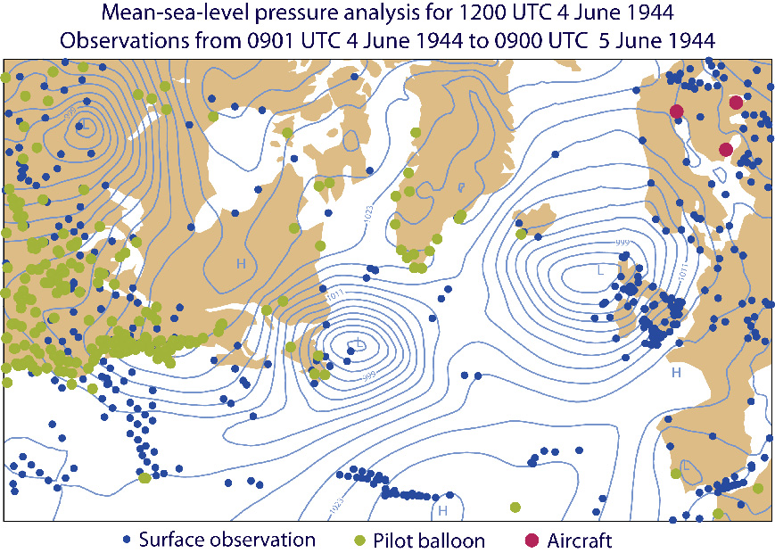
Figure 3 Locations of observations assimilated between 0901 UTC 4 June and 0900 UTC 5 June 1944, superimposed on the surface pressure analysis (contour interval 3 hPa) for 1200 UTC 4 June.
This is very far from all of the data available. Aside from the absence of surface data over occupied France, a quite considerable amount of upper-air data over and close to Europe remains to be digitised and entered into new versions of the databases. Indeed, as a member of the US forecasting team in 1944, Robert Bundgaard, wrote in the report of the 1984 AMS symposium: “By D-Day there was a very considerable amount of upper-air weather information available. The coverage was not as bad as thought.” These data come not only from balloon ascents but also from reconnaissance flights that included profile information from ascents and descents. Some of the paper records containing these data have been scanned, for example the UK Daily Weather Report and the German Täglicher Wetterbericht, but their contents remain to be digitised. Some of this will be done in ERA-CLIM2, but much more will remain to be completed afterwards.
A dearth of observations is nevertheless likely to remain over the central North Atlantic – a challenge for the making of accurate analyses and forecasts in 1944, and still so today. Essentially, the digitised observations available for present use describe conditions at the lateral and lower boundaries of the Atlantic. The numerous pilot-balloon ascents provide control of the data assimilation around much of the periphery of the North Atlantic, especially upstream over North America, while the observations from ships provide limited control at the surface. The assimilating numerical model of the atmosphere completes the picture in the approach we now can use.
Tracking the course of the invasion fleet
Sufficient surface observations are contained in the databases to track the course of the invasion on 5 and 6 June. The surface observations plotted in Figure 4 show elements of the fleet setting out from Southwest England on the morning of the 5th and moving up the Channel in the afternoon. By the evening of the 5th observations are reported from ships at various stages of their journey across the Channel towards Normandy. The absence of observations from occupied France is striking, but observations from Jersey are available for all but the night-time hours.
Observations are not surprisingly fewer in number around the time of the initial landings. Later on 6 June, they are clustered along the Normandy shoreline. All observations from Normandy in these maps are nominally from ships, and at least some of those located inland on these maps are without doubt due to errors in the positions assigned to the observations in the ICOADS database. The observations circled in red in Figure 4 are a case in point. Further discussion can be found in Annex 1.
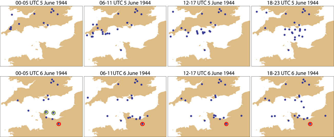
Figure 4 Locations of assimilated surface observations for six-hour intervals from 5 and 6 June 1944.
What type of observation is available for the time the assault began? We have examined the reports from the two ships whose positions are denoted by green circles in the map for 00-05 UTC on 6 June shown in Figure 4. They both come from ships of the same class, HMS Frobisher and HMS Hawkins, two heavy cruisers assigned initially to undertake bombardment of shore defences on D-Day. Figure 5 shows both the digitised observational record in converted units as retrieved from the ICOADS database, and the data (in brackets) as recorded in the original logs, with temperatures in degrees Fahrenheit, winds reported in terms of points of the compass and force on the Beaufort scale, and the character “c” denoting the state of the weather to be cloudy.
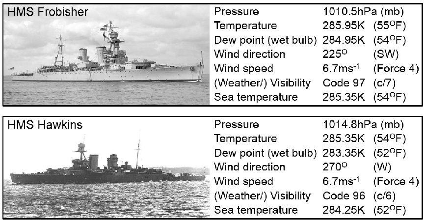
Figure 5 Observations recovered from the deck logs of HMS Frobisher and HMS Hawkins for 02 UTC 6 June 1944. Photographs are from the Royal Naval Museum and uboat.net.
The observations shown in Figure 5 were made at 4 am local time (02 UTC), about two and a half hours before the first landings on Omaha and Utah beaches. The log for HMS Frobisher (Figure 6) shows that it was in fact at 4 am that the call was made to action stations. The log makes sobering reading, as remarks relating first to bombardment and then to the passage of landing craft, to casualties and to loss of life are interspersed with the four-hourly weather reports. The log also shows that the port of departure of the ship was Greenock, in Scotland, and how the ship’s subsequent location was formally recorded at eight-hourly intervals, less frequently than the weather. Further discussion can be found in Annex 1.
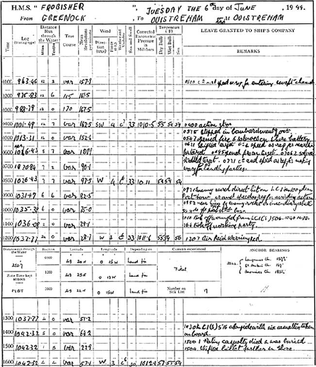
Figure 6 Extract from the deck log of HMS Frobisher for 6 June 1944, copied from the UK National Archives, from which meteorological data were digitised by the US National Climatic Data Center (NCDC) under its Climate Database Modernization Program. Times are Double British Summer Time, two hours ahead of UTC. Eric Freeman, of NCDC, is thanked for facilitating access to these and similar logs.
Surface maps
Figure 7 shows weather maps for 1, 2 and 3 June 1944 from our analyses, for what today is the standard analysis time of 12 UTC, and reproduced from Stagg’s book for 13 UTC, the standard analysis time in 1944. Figure 8 shows corresponding maps for 4, 5 and 6 June. Stagg’s maps show surface pressure with a contour interval of 3 hPa and a depiction of linked frontal structures that appears unfamiliar to modern eyes. We present corresponding plots of surface pressure from our analyses, and depict by arrows the strength and direction of the wind at 10 m height. Strong gradients in wind strength and sharp shifts in direction denote the presence of frontal zones that can generally be identified with what is marked at similar locations on Stagg’s charts.
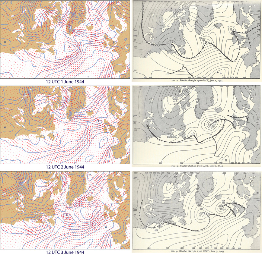
Figure 7 12 UTC ERA-CLIM analyses of surface pressure and ten-metre wind (left) and 13 UTC surface-pressure analyses from Stagg’s book (right), for 1, 2 and 3 June 1944 (upper, middle, bottom). The contour interval for surface pressure is 3 hPa.
The first three days of June 1944 were characterised by quite small-scale depressions strung across the Atlantic from Newfoundland to the north of Scotland, with a tongue of high pressure extending from the Azores towards the South-West Approaches and the Bay of Biscay. The basic features are seen both in Stagg’s maps and in ours, although differences of detail are quite apparent. The same is true, however, of comparisons of Stagg’s maps with Met Office maps produced at the time, as discussed further in Annex 2.
Stagg’s book describes how, at the conferences of the forecasting teams held on the evening of 3 June and early on 4 June, discussion centred on the likely eastward movement of the low west of Scotland, and the extent to which the associated region of strong winds west and south-west of Ireland, and accompanying cloud, would move into the Channel and disrupt the landings planned for the 5th. There was also discussion of the development and movement across the Atlantic of the depression forming near Nova Scotia, and of how much it would directly influence conditions over the Channel at a later stage. At the subsequent briefings of Eisenhower and his commanders at their headquarters outside Portsmouth, Stagg presented the view that conditions in the Channel would worsen during 4 June, and not improve until a cold front passed through. This was estimated to be on 7 June at the evening briefing on the 3rd, but brought forward 24 to 36 hours at the briefing early on the 4th. The decision to postpone the landings was taken provisionally at the evening meeting, and confirmed in the morning, when the weather was still fine over Southern England.
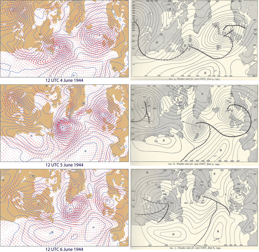
Figure 8 12 UTC ERA-CLIM analyses of surface pressure and ten-metre wind (left) and 13 UTC surface-pressure analyses from Stagg’s book (right), for 4, 5 and 6 June 1944 (upper, middle, bottom). The contour interval for surface pressure is 3 hPa.
From 3 to 5 June, the low west of Scotland not only moved eastward but also developed in depth and scale, as did the low that had formed near Nova Scotia. These systems are depicted similarly in the two sets of maps shown in Figure 8. Reductions in intensity and southward movement of the low over the North Sea by 6 June can also be seen to be generally similar, but there are differences for the low south of Greenland. A third substantial low-pressure system, over North America, is located rather differently in the maps for the 4th, but becomes more similar in the analyses for the subsequent two days. By the evening of 4 June, the intensification of the low passing north of Scotland was foreseen to bring an earlier and stronger clearance of conditions in the Channel. This, together with the predicted slowing of the mid-Atlantic low, offered the window of opportunity that enabled the military decision to be taken to proceed with the landings on the 6th, even though conditions were likely to be some way short of the ideal.
Stagg’s book contains descriptions of what was forecast in the days leading up to 6 June, but no forecast charts with which to compare. Figure 9 shows the ERA-CLIM forecasts for 12 UTC on 5 June made from analyses for 36 h, 60 h and 84 h earlier. They are compared with the analysis for 13 UTC on 5 June from Stagg’s book. The forecasts at the ranges of both 36 h and 60 h successfully capture the development as well as the movement of the low centred north-east of Scotland. Although eastward progression of the storm is a little slow in the 60 h forecast, which was initiated from the analysis for 00 UTC on 3 June, had this forecast been available to the Allied commanders on the afternoon of 3 June, it would have supported a decision to postpone the landings planned for the 5th.
The same cannot be said of the forecast at 84 h range initiated from the analysis for 00 UTC on 2 June. This indicated a much weaker low north of Scotland and a different development further west. Conditions for the Channel were predicted to be more benign than in subsequent forecasts.
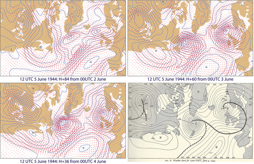
Figure 9 ERA-CLIM forecasts at 84 h (upper left), 60 h (upper right) and 36 h (lower left) range, all valid at 12 UTC 5 June 1944, and the 13 UTC analysis of surface pressure for 5 June from Stagg’s book.
Figure 10 shows the corresponding forecasts for 12 UTC on 6 June. In this case forecasts at all three time ranges capture the essential development of the synoptic situation, with largest difference from Stagg’s map south of Greenland at all ranges. The forecast at 84 h range has too intense a low in the North Sea, and would have cast doubts on an invasion on the 6th had it been available in 1944. The later forecasts predict conditions over the Channel more-or-less as occurred.
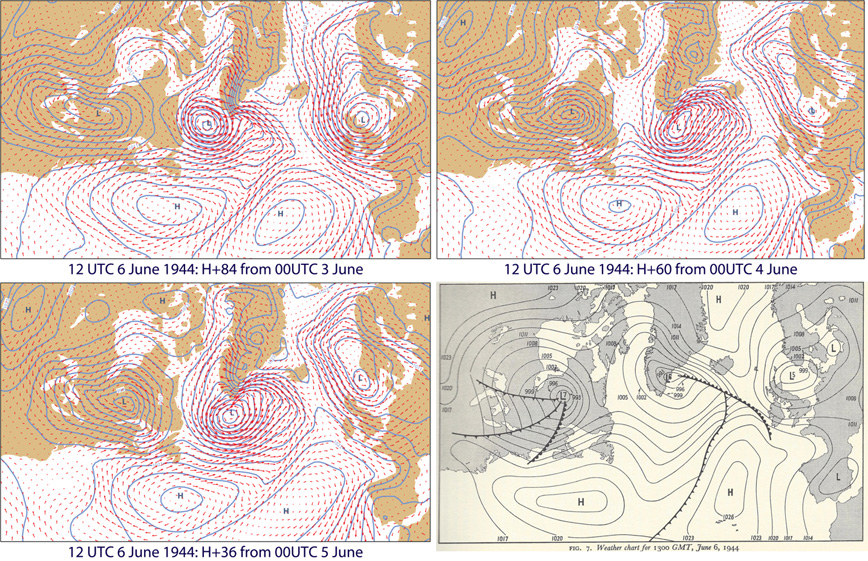
Figure 10 ERA-CLIM forecasts at 84 h (upper left), 60 h (upper right) and 36 h (lower left) range, all valid at 12 UTC 6 June 1944, and the 13 UTC analysis of surface pressure for 6 June from Stagg’s book.
Contemporary British and German analyses for the morning of 6 June are shown in Figure 11, along with the 9h ERA-CLIM forecast from midnight. The Met Office had access for much of the time to de-cyphered German meteorological data (Lewis, 1985, Meteorological Magazine), but none are marked on the chart shown. The German chart shows no observations over the United Kingdom or Ireland. The different styles used for drawing charts are also evident. ERA-CLIM provides a distribution of surface pressure over Western Europe that is in general agreement with both the contemporary analyses. It places the low that by this time is filling over the North Sea closer to the position given in the British analysis, but the low has a central pressure higher than in both other analyses. Further discussion can be found in Annex 3.
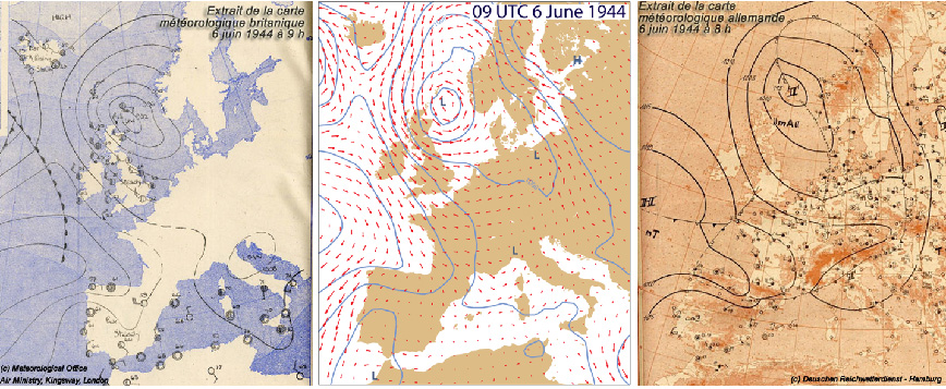
Figure 11 Contemporary British (left; contour interval 4 hPa) and German (right; contour interval 5 hPa) surface pressure analyses for the morning of 6 June 1944, copied in June 2004 from a 60th-anniversary item on the Météo-France website. Corresponding surface pressure (contour interval: 4 hPa) and 10-metre winds from a 9h ERA-CLIM forecast from 00 UTC 6 June are shown in the central panel.
Wind and cloud
We now compare wind and cloud conditions from high-resolution short-range forecasts with what is seen in documents and photographs for 5 to 8 June.
It was at a meeting at the headquarters near Portsmouth starting at 0415 am local time on 5 June that the decision to proceed with the landings on 6 June was confirmed. In his book, Stagg recalls using the words “The fair interval that has reached here ...” in his briefing. Our high-resolution forecast valid shortly afterwards (Figure 12) shows overcast conditions and winds that are quite strong over much of the Channel. Clearance from the north-west of what in reality was the storm that prevented the landings from taking place on the 5th can be seen, but occurs a little later than can be inferred from Stagg’s account. The forecast for 15 UTC shows a subsequent increase in wind and cloud over the South Coast of England that matches conditions that worried Stagg later in the day.
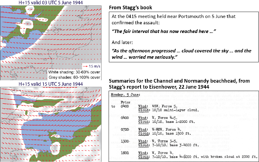
Figure 12 Cloud cover and 10m wind for 5 June 1944 from short-range high-resolution (~16km grid) forecasts carried out from ERA-CLIM analyses, and extracts from Stagg’s book and a report Stagg made to Eisenhower.
Also included in Figure 12 is a summary of the weather over the Channel and Normandy beachhead for 5 June copied from a set included in a report that Stagg delivered to Eisenhower a little over two weeks later. It records west-south-westerly winds at Force 5 and full cover by multi-layer cloud for the early hours of the day. Winds in general weaken a little during the course of the day, but are reported as Force 4 in the evening, when many ships had set out across the Channel. The reported cloud amounts later in the day are greater than in our short-range forecasts.
Figure 13 relates to the early morning of 6 June. The forecast winds strengthen over this period, shifting from longshore to slightly onshore near the Normandy coast, and becoming north-westerly over much of the Channel. The associated cloud starts to clear over the Channel, and is partial over the invasion beaches. Stagg reports “Beachhead clear, with low cloud inland” at 0545, but the two upper photographs give a dark view of the approach to Omaha beach. The wind direction is evident from the smoke plume seen in the lower photograph.
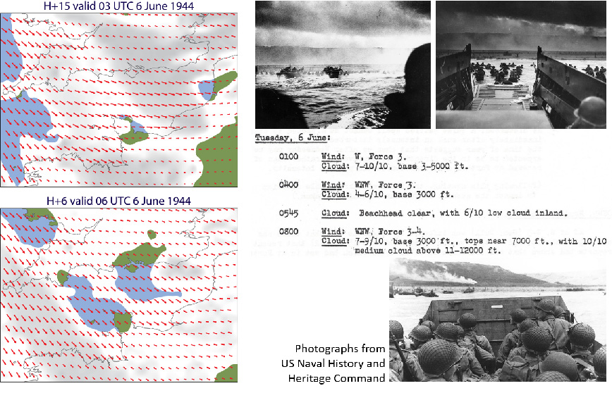
Figure 13 Cloud cover and 10m wind for the morning of 6 June 1944 from short-range high-resolution forecasts, extracts from Stagg’s report to Eisenhower and photographs of the approach to Omaha Beach.
The ongoing clearance of cloud over the Channel seen in the maps presented in Figure 14 matches what Stagg reports for the late forenoon. The upper photograph shows Canadian troops disembarking with bicycles at Nan White beach in conditions that are still cloudy shortly before midday, but many photographs provide evidence of afternoon sunshine, such as the two lower ones showing contact between British troops and local residents. The first synoptic report from Normandy received by the Met Office, from Sword Beach at 13 UTC, was of mainly sunny weather and a north-westerly wind at Force 4.
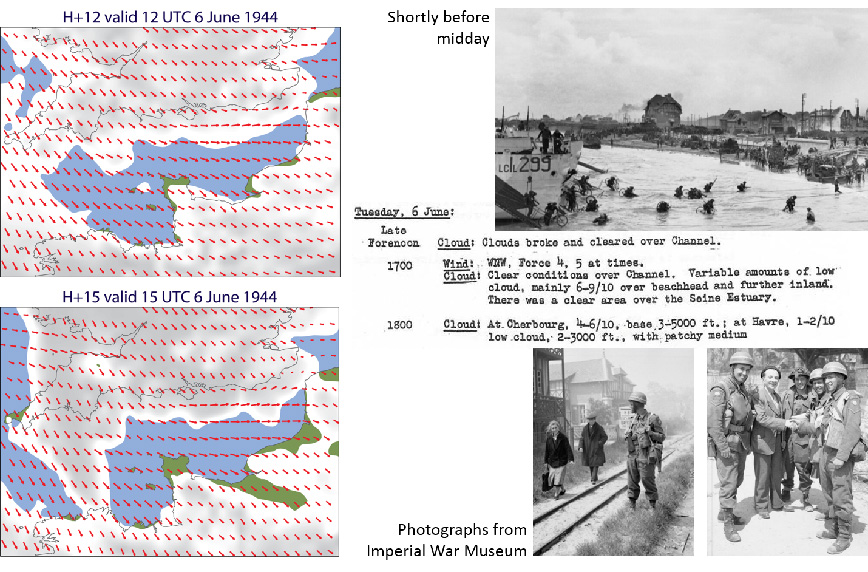
Figure 14 Cloud cover and 10m wind later on 6 June 1944 from short-range high-resolution forecasts, extracts from Stagg’s report to Eisenhower and photographs of Canadian and British troops.
The extent to which conditions would be favourable for reinforcement on the days following the initial landings was another uncertainty at the time the invasion was confirmed. In the event, our short-range forecasts (Figure 15) show weaker winds, northerly on 7th June. This is confirmed by examining synoptic reports from the South Coast of England and inspection of the corresponding maps in the UK Daily Weather Reports, and from the conditions recorded in the logs of HMS Frobisher and HMS Hawkins off the Normandy coast. It does, however, differ rather from the windier picture portrayed in Stagg’s report to Eisenhower, especially for later in the day on the 8th. Our analyses do, however, depict the build-up of stronger, south-westerly winds and clouds on the English side of the Channel on the afternoon and evening of the 8th, with winds remaining low off the Normandy shore. Log entries for 18 UTC are “Light airs” from HMS Frobisher and Force 3 from HMS Hawkins. Evidently this was an occasion when wind conditions over the Channel and the Normandy beachhead could not be summarised as succinctly as the format of Stagg’s report to Eisenhower allowed.
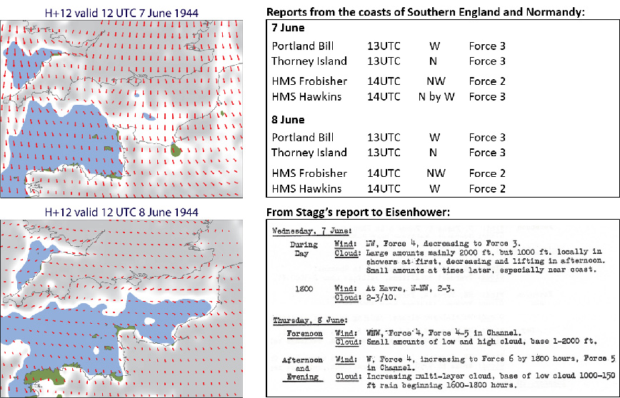
Figure 15 Cloud cover and 10m wind for 12 UTC on 7 June and 8 June 1944 from short-range high-resolution forecasts, selected reports of winds from the coasts of Southern England and Normandy, and extracts from Stagg’s report to Eisenhower
Sea-state
Sea-state conditions have been simulated by using a succession of high-resolution wind forecasts at ranges 6 h, 9 h, 12 h and 15 h to drive a version of ECMWF’s ocean-wave model with 11 km grid resolution. Figure 16 presents an animation of significant wave height, the average trough-to-crest height of the highest third of waves, for the period from 2 to 7 June. Swell is taken into account. The animation shows decreasing wave heights in the Channel from 2 to 3 June, followed by an increase associated with the passage of the storm that in reality delayed the invasion. A general decline starts on 5 June and continues on 6 and 7 June.
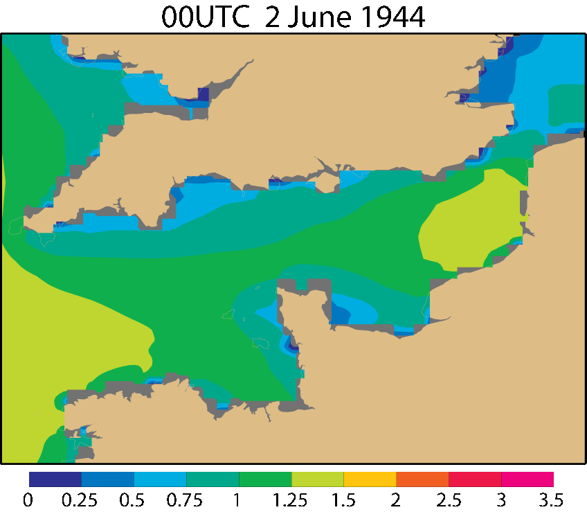
Figure 16 Significant wave height (metres) for 2 to 7 June from a wave model with 0.1o grid, driven by winds from successive 6h, 9h, 12h and 15h forecasts, produced 12 hourly.
Maximum wave heights are typically about double significant wave heights. This is confirmed in this case, as the modelled waves have maximum heights in the range 3-4 m in the Channel over the night of 4/5 June. They drop to 2-3 m during the 5th, apart from an afternoon increase above 3 m linked to the wind intensification noted by Stagg. Maximum heights remain above 2 m in the middle of the Channel on 6 June, with maxima off the Normandy beaches increasing above 1m during the morning as winds strengthen a little and shift to north-westerly, reducing the sheltering effect of the Cotentin Peninsula. Maximum heights drop below 2 m in the middle of the Channel during the early hours of 7 June, and are below one metre over the route between the Isle of Wight and Normandy by late evening, associated with the weaker, northerly winds, with shorter fetch.
The upper air
We conclude consideration of the period around D-Day itself with a brief look at conditions aloft. Figure 17 compares the ERA-CLIM 500 hPa height analyses for 12 UTC on 4, 5 and 6 June with copies of the original 13 UTC Met Office charts for these days that were presented by Karl Johannessen in the 1984 AMS publication illustrated in Figure 1. Johannessen was a visitor for a while in the then Operations Department of ECMWF during the early days of the Centre at Shinfield Park. He recalled in his article that he was working at the Met Office forecasting centre at Dunstable in June 1944.
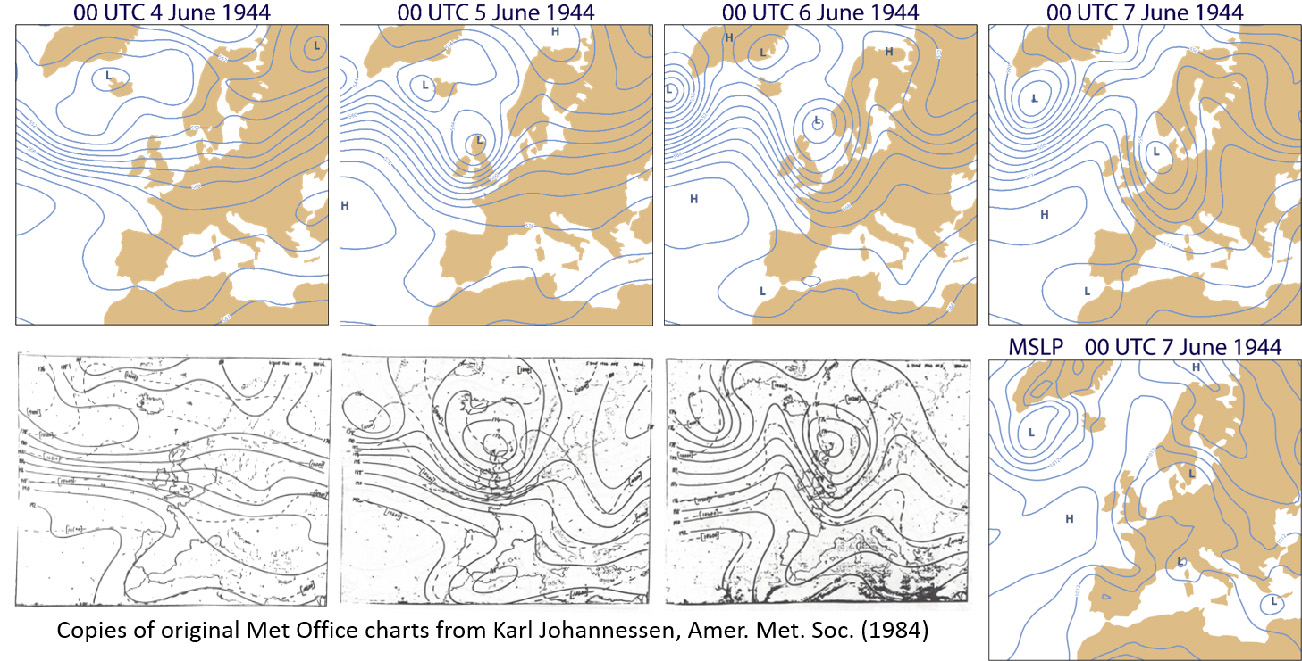
Figure 17 ERA-CLIM 500 hPa height analyses (contour interval: 60 m) for 00 UTC 4 to 7 June 1944, and contemporary Met Office analyses (contour interval: 200 ft) for 4 to 6 June. The ERA-CLIM surface-pressure analysis (contour interval: 4 hPa) is also shown for 7 June.
Although our analyses do not benefit from assimilation of most of the upper-air data available for Western Europe and the Eastern Atlantic for the period, the data assimilation system is capable nevertheless of producing 500 hPa charts that are in good agreement with those produced at the time. We carry the picture beyond 6 June in Figure 17 by showing both the 500 hPa and the surface analysis for 12 UTC on 7 June.
How important were such upper-air charts for the forecasting process? Accounts differ. Johannessen wrote in 1984: “What did we know about development, and how did the upper-air maps help us tell what was going to happen near the surface? The answers are very, very little.” In contrast, Robert Ratcliffe wrote in a letter published in the same volume: “… we in the upper air section [of the Met Office] were able to convince the surface forecaster … that the strong diffluent upper thickness pattern in the Atlantic and what would now be called a westerly jet stream with its left exit approaching the U.K. [seen in the map for 4 June] would mean the depression deepening and probably stagnating near north Britain.”
However, it was not until the post-war years that processes such as downstream dispersion and development, and meridional trough extension and deceleration following amplification of an upstream ridge, became understood and translated into forecasting rules. The southward movement over the North Sea of the surface depression and closed low at 500 hPa from 6 to 7 June depicted in Figure 17 was indicated in none of forecasts discussed by Stagg in his book. Instead, as the decision was made to proceed with the landings on 6 June the expectation reported by Stagg was for westerly or south-westerly winds over the Channel, strong at times, on 7 and 8 June. Stagg commented in hindsight that the unexpected movement made the initial landings more difficult than expected due to quite strong north-westerly winds on the 6th, but was of overall benefit as conditions on the 7th and for most of the 8th were more favourable for follow-up operations.
The storm of 19-22 June 1944
Had the decision not been made to go ahead with the landings on 6 June or thereabouts, the next occasion when the tides would have been favourable was almost two weeks later. Stagg wrote in his book: “On the evening of June 17th a ridge of quiet weather ... encompassed almost the whole of the British Isles. On the face of it, it looked like the ideal weather set-up for the start of a great invasion, and the outlook seemed favourable for several days. During June 18th, however, two unexpected things happened … .” A member of the Admiralty forecast team, Lawrence Hogben, expressed it this way in a letter to the magazine Weather in June 1994: “We were also lucky because for the alternative invasion date of the 19th each centre forecast calm anticyclonic conditions from the 17th.”
Figure 18 provides observations and images of what happened next along the Normandy shore. A strong north-easterly wind developed and blew at Force 6 or above from the 19th to the 22nd. Its long fetch over the North Sea and Channel resulted in days of high waves that damaged the Mulberry harbour at Omaha Beach beyond repair, and damaged also the surviving Mulberry at Arromanches.
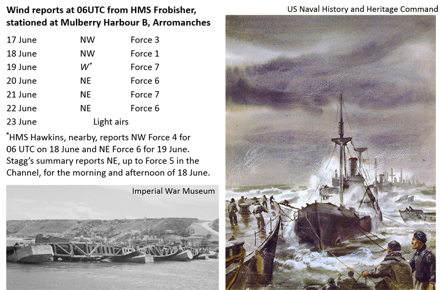
Figure 18 Wind reports and images for the storm of 19-22 June 1944. Images are from the Imperial War Museum and the US Naval History and Heritage Command.
The upper air: 15 to 23 June 1944
We reverse the order of discussion for this event, and consider first the rich set of developments analysed for the upper air. Daily maps of 500 hPa height from 15 to 23 June are shown in Figure 19. An alternative view for the atmospheric dynamicist is given in Figure 20, which presents corresponding maps of potential vorticity on the 330 K isentropic surface.
The 500 hPa maps show the development and eastward movement of a pronounced trough over the Western Atlantic, and the development of the ridge ahead of it. The trough decays and a strong jet is established at northern latitudes. Meanwhile, a short-wave perturbation west of Scotland on 16 June amplifies and extends southward, cutting off over the Mediterranean. An anticyclone forms to the north of it, amplified apparently by downstream development along the jet to the north. Flow from the north-east is implied over the Channel from 19 June onwards.
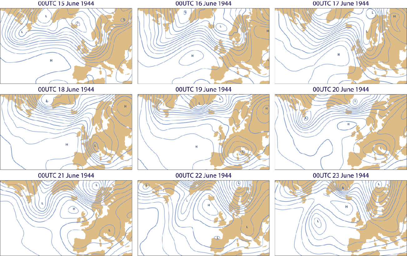
Figure 19 ERA-CLIM 500 hPa height analyses (contour interval: 40 m) for 00 UTC from 15 to 23 June 1944.
The potential vorticity maps provide a sharper picture of events. We are unable to vouch for the veracity of some of the details given the limited availability of upper-air observations for assimilation, but development appears to be consistent from day to day and with what is seen in the 500 hPa height field. We comment specifically only on the map for 19 June. The two “unexpected developments” around 18 June referred to by Stagg in his book were the rapid south-eastward movement of a cold front from Iceland towards the British Isles, with high pressure building behind it, and the formation of a depression over the Mediterranean that spread northward over France and deepened. The frontal movement is presumably linked with the thinning remnant of the tongue of high 330 K potential vorticity located earlier over the Western Atlantic (associated with the trough in 500 hPa height) that can be seen over Scotland at 00 UTC on 19 June. Surface cyclogenesis over the Mediterranean accompanies the southward movement of the downstream tongue of high potential vorticity air (and the development of the cut-off in the 500 hPa height field).
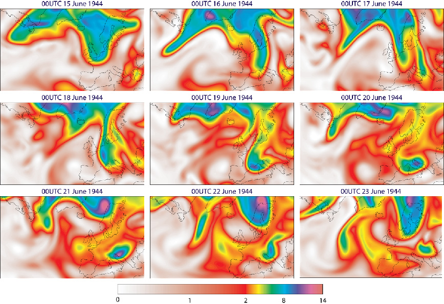
Figure 20 ERA-CLIM analyses of potential vorticity (10-6 m2 s-1 K kg-1) on the 330 K isentropic surface for 00 UTC from 15 to 23 June 1944.
Surface maps: 16 to 23 June 1944
Daily surface-pressure analyses over Western Europe from 16 to 23 June are shown in Figure 21. A weakening low over Scotland on 16 June moves south eastwards over Denmark and into Northern Germany, as a new low develops over the Gulf of Genoa, moving eastward and then northward as described by Stagg. Instead of the calm anticyclonic conditions after the 17th expected by the forecasting teams , a strong and persistent gradient in surface pressure developed over the southern North Sea and Channel, and bordering countries, weakening only towards the end of the period.
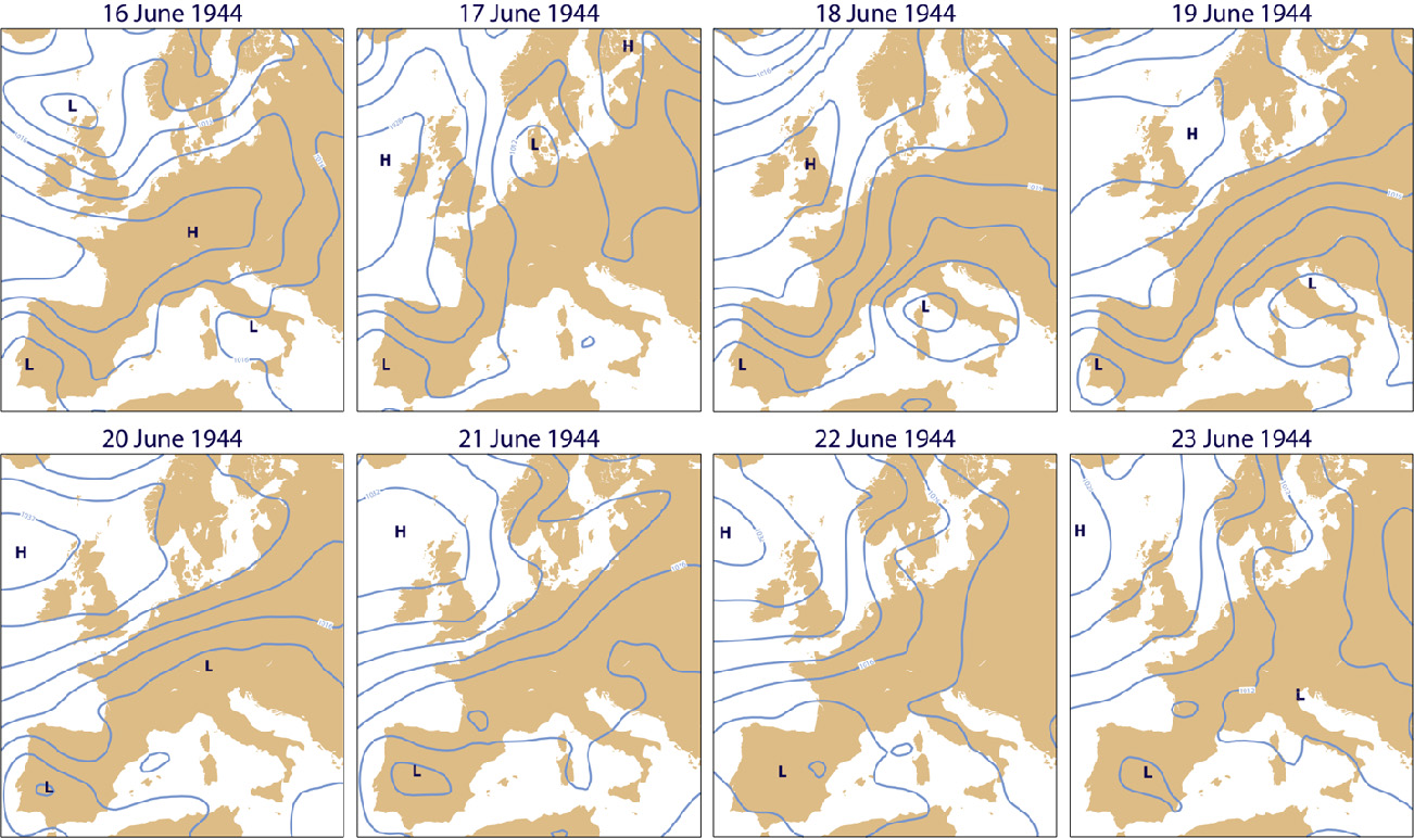
Figure 21 ERA-CLIM surface-pressure analyses (contour interval: 4 hPa) for 00 UTC from 16 to 23 June 1944.
In this case the forecasts run from these analyses as part of ERA-CLIM show how modern-day forecasting would have provided an alert several days in advance, even with the observing system of the time. Figure 22 is a mosaic of surface-pressure maps from forecasts for 19, 20, 21 and 22 June initiated one, two, three and four days ahead of time. The forecasts evidently degrade in detail as their range increases, and tend to underestimate the intensity of the main pressure gradient, but they capture the essential nature of the development despite limitations in observational coverage and model resolution.
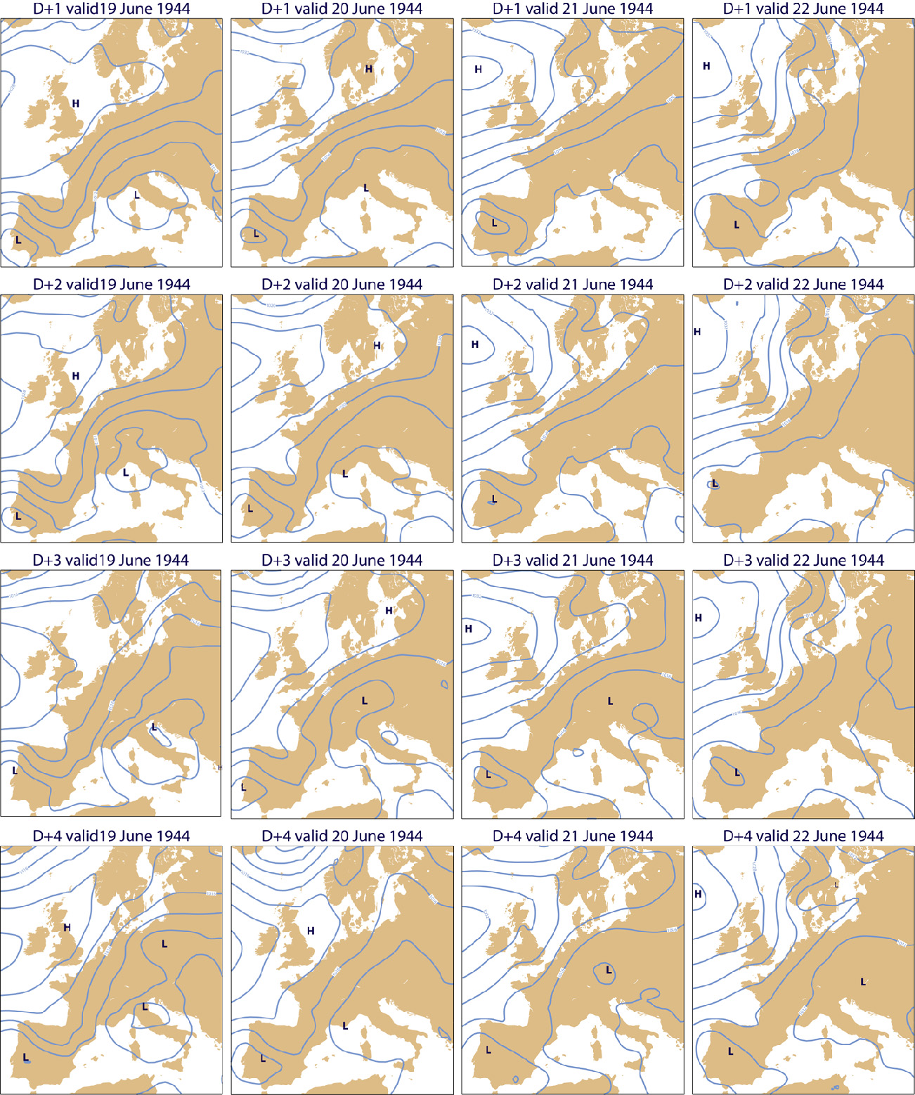
Figure 22 ERA-CLIM surface-pressure forecasts (contour interval: 4 hPa) for 00 UTC from 19 to 22 June 1944 at ranges from one to four days ahead.
Wind, cloud and sea-state: 18 to 23 June 1944
High-resolution forecasts have been run for this period, and maps of wind and cloud are shown twelve-hourly at 6 h forecast range in Figure 23. The persistence of the north-easterly flow onto the Normandy shore is striking. Cloud comes and goes over the Channel, with only limited agreement with the summaries provided (up to 21 June) in Stagg’s report to Eisenhower, which was dated 22 June. Cloud is more persistent along the Normandy coast. Winds are strongest on the evening of 20 June, when they reach almost 15 ms-1, or Beaufort Force 7. They are much weaker by the morning of 23 June. They re-intensify later in the day, though this is not reflected in the evening observations of “Light airs” by HMS Frobisher and Force 2 by HMS Hawkins.
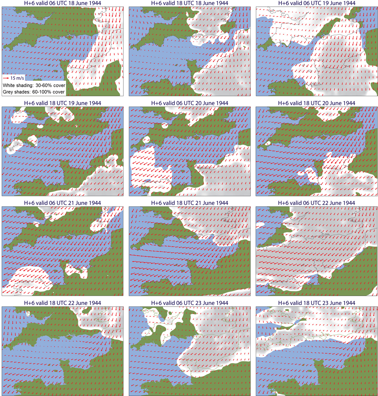
Figure 23 Cloud cover and 10m wind from short-range high-resolution forecasts for 06 and 18 UTC from 18 to 23 June 1944.
The long fetch of winds from the North Sea, through the Dover Strait and along the Channel to the Normandy shore drove waves of considerable height onto the beaches and harbours. A US Naval Report on the storm refers to “wave action of eight to ten feet” and a memoir dated 2010 written by one of the forecasters responsible at the time for predicting sea, swell and surf, Charles Bates, notes: “Off Omaha … the USS Augusta … [reported] … maximum wave heights of 12 feet …”
Figure 24 is an animation of significant wave heights for 18 to 23 June, produced in the same way and using the same colour scale as the animation for 2 to 7 June presented in Figure 16. Values exceed 1.5 m off the Normandy shore continuously from the evening of 19 June to the evening of 22 June, and just exceed 2.5 m at 18 UTC and 21 UTC on 20 June. Values fall below 1 m on the morning of 23 June before rising later. Maximum wave heights are again around twice the significant wave heights, reaching as high as 5 m at the eastern end of the Normandy beaches at 18 UTC on 20 June, and 4 m close to Omaha beach at this time.
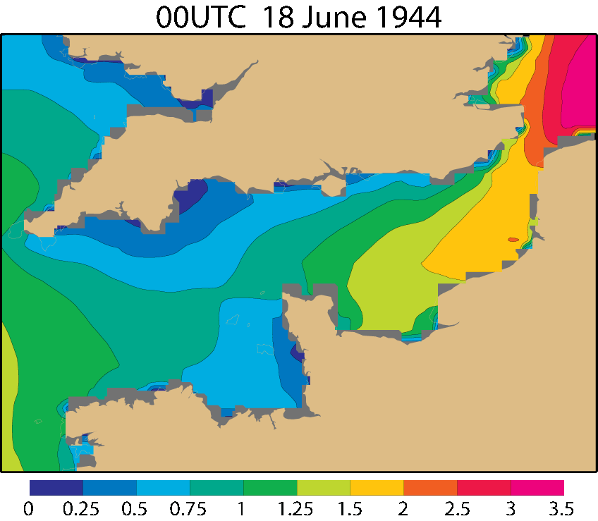
Figure 24 Significant wave height (metres) for 18 to 23 June from a wave model with 0.1O grid, driven by winds from successive 6h, 9h, 12h and 15h forecasts, produced 12 hourly.
Improvement on our first analyses for June 1944
The analyses for June 1944 made in 2004 were a quick, one-off effort, using the ERA-40 assimilation system without adjustment for the diminished number and quality of observations. Observations were restricted to a single source, and absence of a readily usable sea-surface temperature analysis led us to use the values from one particular year from the ERA-40 period. Analyses made in 2014 were part of a long-term programme of climate reanalysis, with purpose-designed modifications of the data assimilation system and a much more comprehensive set of observations assimilated, using an analysis of sea-surface temperature for June 1944.
Our analysis ten years ago captured the broad synoptic situation of both the D-Day period and the storm two weeks later. Conditions over Normandy on D-Day itself were fairly realistic, but had too predominant a westerly component to the wind field. The principal developments in the Atlantic were delayed, however, and at the time of the landings the low that in reality was located over the North Sea extended from the west of Scotland to between Iceland and Norway. The cold front that in reality and our recent analyses cleared the channel in the morning of 5 June stalled and decayed in the west of the Channel. This was viewed as a reasonable first attempt, but it was clear that with effort we could do better. Figure 25 presents surface maps for 12 UTC on 4 and 6 June from our original and recent analyses, and the corresponding maps from Stagg’s book.
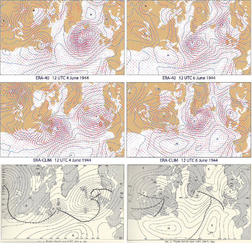
Figure 25 Analyses of surface pressure and ten-metre wind for 12 UTC on 4 June (left) and 6 June (right) from an initial analysis for the D-Day period carried out in 2004 using the ERA-40 assimilation system (top). Corresponding maps are shown for the latest ERA-CLIM analyses (middle) and the 13 UTC surface-pressure and frontal analyses from Stagg’s book (bottom). The contour interval for surface pressure is 3 hPa.
Concluding remarks
Writing some twenty-five years after the event, Stagg questioned in a postscript to his book whether the advances in weather prediction over the intervening period, had they been in place in 1944, would have affected the advice he gave to Eisenhower. He believed not, citing that although there was difficulty during the war in collecting weather reports from the North Atlantic, information from the region was still not enough to allow regular and reliable forecasting beyond 24 hours. He also cited what he considered to be the inherent unpredictability of the atmosphere after a day or two.
Forty-five or so years later we have witnessed and been part of a tremendous advance in our capability to forecast the weather. In part this is due to the availability of satellite data that now give us several different views of conditions over the oceans and lands of the world. But it is also due to advances in understanding, advances in modelling and data assimilation, and advances in the computing technology needed for implementation. These advances, allied with efforts to recover historical data and build digital archives, have enabled us to present evidence to address again the question that Stagg raised. Readers may form their own views as to the answer.
From our perspective, the expectations we had at the outset of our second reanalysis of the D-Day period have been met or exceeded. We are now able to produce analyses that in general terms match those reported by Stagg, and that are a matter for discussion where disagreement can be seen. Our forecasts, even when penalised for starting from analyses that used observations taken several hours later, do depict the essentials of the evolution of the critical weather systems in June 1944 for 48 hours or longer ahead, despite the limitations of the observations used. The detail cannot be perfect, however, and variables such as cloud that remain today a challenge in some types of synoptic situation are yet more of a problem with the observations available from seventy years ago. And what we can do today in the quiet of our offices or even connected through the internet from the comfort of home should in no way detract from the achievements of Stagg and his colleagues under a very different set of circumstances.
Stagg noted in his book that the low that crossed northern Scotland on the night of 4/5 June 1944 led to the lowest surface pressure, 976.8 hPa, recorded over the British Isles in any June [to date] in the 20th Century, and that disturbed weather prevailed for much of the summer and autumn that year. As reanalysis progresses, and attains a capability to reproduce such extremes and sequences of weather, it provides new opportunities to put these events in a long-term climatological context and explore the mechanisms involved.
Improvement will continue in our capability to reanalyse periods such as June 1944. This will come from better modelling and data assimilation, where improvement is already known to be possible in principle as existing efforts have involved compromises due to limitations in the availability of computing resources. It will come from better quality control and correction of existing data holdings, addressing problems such as have been identified here in some of the observations for June 1944. And it will come from the recovery of additional data, where all can make a small contribution through participating in crowd-sourced digitisation initiatives such as Old Weather and Data Rescue at Home.
Annex 1
The locations of ship observations and the track of HMS Frobisher in June 1944
Although the majority of observations identified as from ships in the databases used by ERA-CLIM are located over the open oceans or coastal waters, a number of instances have been found in which the observation has been assigned a location over land, in a position that cannot be explained by the vessel being on an inland waterway. On occasions this could be due to a genuine observation over land being reported as if from a ship. However, when the source of the observation is well known to be a ship, this indicates an error in digitisation that may be corrected for future use of the data. We illustrate this for two cases.
The first is a set of observations available at intervals during 6 June located at precisely 49ON on the Greenwich meridian, well south of the Normandy coastline, circled red in Figure 4 . They are from the digitised deck log of HMS Argonaut, a light cruiser that on 6 June was at sea off the Normandy shore, providing gunnery support for the British landings on Gold beach. The log itself does not record locations in routine format that day, but includes remarks that that the ship’s location was 50O 0/N, 0O38½/W at 0216 Double British Summer Time (DBST) and at 49O27/N, 0O40/W at 0500 DBST, the latter being described as its “bombarding position”.
The second concerns HMS Frobisher. The extract from its deck log reproduced in Figure 6 shows that as a matter of routine, the location of the ship was recorded three times per day, less frequently than the weather. As was also the case for HMS Argonaut and all other Royal Navy vessels whose digitised weather data are found in the ICOADS database, the locations of the ship at the times the individual weather observations were made had to be estimated. In the case of HMS Frobisher, positions for June 1944 appear to be essentially correct for all but one 24-hour period. Figure A1 shows them from 3 June onwards. The sequence of dark blue dots covers the latter part of her journey from Greenock to rendezvous with the invasion fleet south of the Isle of Wight, before proceeding to Normandy where on 6 June she eventually moved close to the shore off Ouistreham, as recorded in the log for the day (Figure 6). Subsequent logs show that she remained in action in the vicinity until the evening of 8 June, when she re-crossed the channel to Portsmouth. Here she was provisioned so as to return to Normandy on 12 June to serve for the rest of the month as a depot ship in Mulberry Harbour B at Arromanches. This sequence of events is captured in the locations shown in Figure S1, apart from a period from late on 7 June when the observation locations correspond to the ship moving southward over land into Normandy before suddenly reverting to a northward course that takes her back to arrive at Portsmouth by the recorded time that this happened. It has since been found that this is because the latitude 49O26/N given in the deck log for 2000 DBST on 8 June was erroneously transcribed as 48O26/N during one stage of the digitisation process.
Figure A1 Observation locations in the database for HMS Frobisher, 3-30 June 1944
The effect of such positional errors on our analyses is mitigated by the presence of neighbouring observations and by the relatively low (about 125 km) horizontal resolution of the ERA-CLIM data assimilation system. Together with inconsistencies in the observations from different ships (Annex 3), this may however explain why a first attempt at analysing the period using the operational (16km) resolution provided results with many more unrealistic-looking, small-scale features than we are accustomed to seeing today in our operational analyses.
Annex 2
Contemporary weather maps for the North Atlantic
The charts presented in Stagg’s book are what he described as “small-scale facsimiles of others which, a week or two after the events to which they relate, were acknowledged by all the people who took part in the discussions as being acceptably similar to their own charts”. He reported that the actual charts he had used in the days leading up to the invasion could not later be found, and noted that the real-time charts used by the three forecasting centres feeding in to the critical consultations must on occasions “have had little resemblance” to the “post-hoc charts” he presented in his book.
To illustrate this, we compare in Figure A2 the surface charts shown in Stagg’s book for 13 UTC on 2, 3 and 4 June with corresponding surface charts presented by Karl Johannessen in the 1984 AMS publication illustrated in Figure 1. Strict comparison is made difficult by differences in map projection and contour interval, but quite pronounced differences can nevertheless be seen in Figure A2. One example concerns the low-pressure system south-east of Greenland on 2 June, for which the weaker circulation in the Met Office chart copied by Johannessen is much closer to that seen in our analysis of the system (Figure 7) , although the forecast performance illustrated in Figure 9 leads us to make no special claim for accuracy of our analyses for this day. Differences become less obvious as the Atlantic systems become larger in amplitude and scale on the following two days, but there are differences of detail, in particular in the extent to which the tongue of high pressure extends into the South-West Approaches and the Bay of Biscay, a feature whose evolution was the subject of disagreement among the forecasting teams at the time. Again, our analyses appear to be closer to those of the Met Office team for this feature. This can also be seen in the early-morning northern hemisphere charts for the period contained in the scanned Daily Weather Reports that have recently been made available online by the Met Office.
Figure A2 Maps of surface pressure for 13UTC on 2 June (top), 3 June (middle) and 4 June (bottom) 1944, reproduced from Stagg’s book (left; contour interval: 3hPa) and from Johannessen’s contribution to the 1984 AMS publication (right; contour interval: 4hPa).
Annex 3
Observations from the Orkney Islands on 6 June
Having seen (Figure 11) that the surface pressure for 09 UTC on 6 June from ERA-CLIM is several hPa higher than either the German or (more so) the British analyses for around that time, we examined the observations available to the data assimilation system from the north of Scotland on the morning of 6 June. The first surprise was that there were multiple observations for the same time and for the same location of 58.9ON, 3.1OW in the databases. It soon became evident that these came from Royal Navy vessels (twelve ships and one surfaced submarine) moored or undergoing trials in the protected waters of Scapa Flow, among the islands of Orkney off the northern coast of the Scottish mainland. The second surprise was the extent of the variation among the observations for a given time, shown for 10 UTC in Table A1.
|
Name |
Pressure |
4-hour change |
Wind |
Temperature |
|
|
Anson |
996.8 mb |
3.0 mb |
NE by N |
2 |
51OF |
|
Duke of York |
996.0 mb |
5.1 mb |
W |
2 |
50OF |
|
Howe |
1009.3 mb |
2.5 mb |
NNW |
4 |
Missing |
|
Indomitable |
1002 mb |
-1.0 mb |
W |
2 |
56OF |
|
Jamaica |
99?.?1 mb |
? |
NNE |
4 |
53OF |
|
Kent |
996.3 mb |
5.2 mb |
E |
3 |
54OF |
|
Khedive |
29.5 in Hg (999.0 mb) |
6.1 mb |
N |
5 |
49OF |
|
Royalist |
996.3 mb |
2.1 mb |
NE |
3-4 |
52OF |
|
Searcher |
29.25 in Hg (990.5 mb) |
5.1 mb |
ENE |
4-5 |
52OF |
|
Sheffield |
991 mb |
1.0 mb |
NE |
1 |
56OF |
|
Striker |
29.22 in Hg (989.52 mb) |
4.1 mb |
NNE |
4 |
49OF |
|
Trusty |
998 mb |
Unavailable |
NE |
2 |
59OF |
|
Victorious |
995.2 mb |
2.7 mb |
NNW |
3 |
51OF |
1Unclear scan, digitised as 990.7, but could be 993.9 or 995.9 2Digitised as 985.3
Table A1 Meteorological observations from deck-log entries for 10 UTC 6 June 1944 of Royal Navy vessels at Scapa Flow, all located at 58.9ON, 3.1OW in the database of digitised observations
The ICOADS data presented to ERA-CLIM show a variation of 24 hPa among the observations for this single place and time. This is reduced to a little less than 20 hPa when allowance is made for an error in converting a report of surface pressure that was originally in terms of inches of mercury, and the bias-correction scheme employed in ERA-CLIM reduces the spread to 17.5 hPa. This remains a substantial difference. Considerable spread can also be seen in Table A1 in the four-hour pressure changes (from 06 UTC to 10 UTC), in the wind strengths and directions, and in the air temperatures.
Faced with such a set of observations, the ERA-CLIM assimilation system has a process of data selection that causes it to follow the observation from HMS Anson in this instance. The raw reported pressure from Anson for 10 UTC is 996.8 hPa, but the assimilated value is bias-adjusted to 1000.5 hPa. This is considerably higher than indicated for this time by the land-based observations from the Royal Naval Air Station at Hatston on the main island of Orkney, which reported 992.1 hPa at 07 UTC and 1001.5 hPa at 13 UTC on 6 June 1944, with three-hourly rises of 1 hPa and 5.9 hPa respectively for the two times. Corresponding winds were NW Force 4 and NE Force 5, and temperatures were 50OF and 53OF (B.J. Booth, personal communication). The observation from Orkney marked on the Met Office chart reproduced in Figure 11 is presumably from Hatston. The observations from this station were not in any of the databases that provided the observations for 6 June assimilated by ERA-CLIM, although data from Aberdeen were available for 00 UTC (997.1 hPa) and 06 UTC (997.5 hPa).
The data from Hatston (and many other UK stations) were recorded in the UK Daily Weather Report at the time, and now can be viewed as hand-written entries in the scans that have recently been made available online by the Met Office. We are aware of no immediate arrangement for digitising these data.